Artificial Intelligence is on the front page of all newspapers those days (often for the wrong reasons…). Of course, AI is not new, the field dating from the middle of last century; neither are cascading neural networks, which I used in the 1990s to predict protein’s secondary structures. However, it really exploded with Deep Learning. Some stories made the news over the years, for instance, DeepMind’s AlphaGo beating a Go’s world champion and AlphaFold solving the long-standing problem of predicting protein’s 3D structures (well, at least the non-flexible conserved parts…). Still, most successes remained confined to their respective domains (e.g., environment recognition for autonomous vehicles, tumour identification and machine translation such as Google Translate and DeepL). However, what brought AI to everyone’s attention was OpenAI’s DALL’E and, more recently, ChatGPT, which can generate images and text following a textual prompt.
OpenAI actually developed many other Deep Learning models, some open source. Among those, Whisper models promise to be a real improvement in speech recognition and transcription. Therefore, I decided to test Whisper on two different tasks: a scientific presentation containing technical terminology, given by a US speaker, and a song containing cultural references, sung by an American singer but with no accent (i.e., BBC-like…).
Lenovo Thinkpad T470 I, no GPU. Linux Ubuntu 22.10 Python 3.10.7 Pytorch 2.0 I used the model for speech recognition in the video editing tool Kdenlive 23.04 (Update 31 May 2023: I was able to run Whisper on Linux Ubuntu 23.04 with Python 3.11.2 and Kdenlive 23.04.1 ; although installing all the bits and pieces was not easy)
Whisper can be used locally or through an API via Python or R (for instance with the package openai), although a subscription might be needed if you already used all your free tokens.
There are five Whisper models.
Models
Parameters
Required VRAM
Relative speed
Tiny
39 M
~1 GB
~32x
Base
74 M
~1 GB
~16x
Small
244 M
~2 GB
~6x
Medium
769 M
~5 GB
~2x
Large
1550 M
~10 GB
1x
Note that these models run perfectly well on CPUs. While GPUs are necessary for training Deep Learning models, this is not the case when using them (although running them on CPU will always be slower because of floating point computations).
As an external “control”, I used the VOSK model vosk-model-en-us-0.22 (just called VOSK in the rest of this text).
NB: this is an anecdotal account of my experience, and does not replace comprehensive and systematic tests, for instance, using datasets such as Tedlium. or LibriSpeech test-clean
I used speech recognition to create subtitles, as it represents the final aim in 95% of my professional transcriptions. Many videos are available to explain how to generate subtitles in Kdenlive, including with Whisper.
Transcription of a scientific presentation
The first thing I observed was the split into text fragments. I noticed that their placement along the timeline (the timecodes) was systematically off, starting and finishing too early. Since this did not depend on the model, the problem could come from Kdenlive.
The length of the text fragments varied widely. VOSK produced small fragments, perfect for subtitles, but cut anywhere. Indeed, VOSK does not introduce punctuation and has no notion of sentence. The best fragments were provided by Tiny and Large. They were small, perfect for subtitles, and cut at the right places. On the contrary, Small produced fragments of consistent lengths, longer than Tiny and Large, and thus too long for subtitles, while the fragments produced by Base and Medium were very heterogeneous, only cut after periods.
The models differed straight from the beginning. Tiny produced text that was much worse than VOSK (if we ignore the absence of punctuation by the latter). “professor at pathology” instead of “of pathology”, a missing “and”, a period replaced by a comma, and a quite funny “point of care testing” transformed into “point of fear testing”! All the other models produced perfect texts, Small, Medium, and Large even adhering to my beloved Oxford comma.
VOSK: welcome today i'm john smith i'm a professor of pathology microbiology and immunology and medical director of clinical chemistry and point of care testing
Tiny: Welcome today, I'm John Smith. I'm a professor at Pathology, Microbiology, Immunology, and Medical Director of Clinical Chemistry and Point of Fear Testing.
Base: Welcome today. I'm John Smith. I'm a professor of pathology, microbiology and immunology and medical director of clinical chemistry and point of care testing.
Small: Welcome today. I'm John Smith. I'm a professor of pathology, microbiology, and immunology, and medical director of clinical chemistry and point of care testing.
Medium: Welcome today. I'm John Smith. I'm a professor of pathology, microbiology, and immunology and medical director of clinical chemistry and point of care testing.
Large: Welcome today. I’m John Smith. I'm a professor of pathology, microbiology, and immunology, and medical director of clinical chemistry and point of care testing.
A bit further, the speaker described blood gas analysers. VOSK can only analyse speech using dictionaries. As such, it could not guess that pH, pCO2, and pO2 represent acidity, partial pressure of carbon dioxide and partial pressure of oxygen, respectively and spell them correctly. It also missed the p in pCO2. The result is still understandable for a specialist but would give odd subtitles.. The Whisper models consider the whole context, and can thus infer the correct meaning of the words. Tiny did not understand pH and pCO2, merging them. All the other models produced perfect texts.
VOSK: [...] instruments came out for p h p c o two and p o two
Tiny: [...] instruments came out for PHPCO2 and PO2.
Base: [...] instruments came out for pH, PCO2 and PO2
Small: [...] instruments came out for PH, PCO2, and PO2.
Medium: [...] instruments came out for pH, PCO2, and PO2.
Large: [...] instruments came out for pH, PCO2, and PO2.
VOSK’s dictionaries sometimes gave it an edge. For instance, it knew that co oximetry was a thing, albeit missing a dash. Only Large got it right here, Base, and Medium hearing coaximetry, and Tiny even hearing co-acemetery!
VOSK: [...] we saw co oximetry system
Tiny: [...] we saw co-acemetery systems.
Base: [...] we saw coaximetry systems.
Small: [...] we saw coaxymetry systems.
Medium: [...] we saw coaximetry systems.
Large: [...] we saw co-oxymetry systems.
Another example is the name of chemicals. VOSK recognised benzalkonium, which was recognised only by Medium. Interestingly, the worst performers were Base, which misheard benzylconium, and Large, which misheard benzoalconium (Tiny and Small heard properly but spelt the word wrong, with a ‘c’ instead of a ‘k’).
The way Whisper Large can understand mispronounced words is very impressive. In the following example, Small and Large are the only models correctly recognising that there are two separate sentences. More importantly, VOSK and Tiny could not identify the word “micro-clots”. The hyphenation is a matter of discussion. While the parsimonious rule should apply (do not use hyphens except when not doing so would generate pronunciation errors), using hyphens after micro and macro are commonplace.
VOSK: [...] to correct the problem like micro plots and and i discussed the injection of a clot busting solution
Tiny: […] to correct the proper microplasks. And I discussed the injection of a clock-busting solution.
Base: […] to correct the problem like microclots and I discussed the injection of a clot busting solution.  (wrong start)
Small: […] to correct the problem, like microclots. And I discussed the injection of a clot-busting solution.
Medium: […] to correct the problem, like microclots, and I discussed the injection of a (wrong start, missed end of sentence.)
Large: […] to correct the problem, like micro-clots. And I discussed the injection of a clot-busting solution.
In conclusion, Whisper Large is the best model, not surprisingly, with the surprising exception of the small mistake on “benzalkonium”.
Transcription of a pop culture song
Adding sound on top of speech, such as music, can throw off speech recognition systems. Therefore, I decided to test the models on a song. I chose a very simple song with slow and clearly enunciated lyrics. And frankly, being a nerd, I relished highlighting those fantastic Wizard Rock scene artists whose dozen groups have been celebrating the Harry Potter universe through hundreds of great songs. I used a song from Tonks and the Aurors entitled “what does it means”.
The first massive observation was that I could not compare VOSK to Whisper models. Indeed, the former is absolutely unable to recognise anything. The “transcription” was made of 27 small fragments of complete gibberish, with barely a few correct words. Only one fragment contained an actual piece of the lyrics: “Everybody says that it’s probably nothing”. However, these words were also identified by all Whisper models.
Now for the Whisper models. The overall recognition was remarkable. On the front of fragment size, only Tiny produced small fragments, perfect for subtitles, cut at the right places. Medium was not too bad. Base and Small produced heterogeneous fragments, only cut after periods. Large produced super short segments, often made up of one word. Initially, I thought this was very bad. However, I then realised that it was perfect for subtitling the song; just the right rate in character per second, very readable.
Something odd happened at the start, with some models adding fragments while there was no speech, such as “Add text” (Tiny) or “Music” (Base). Large added the Unicode character “♪” whenever they were music and no speech, which I found nice.
When it came to recognise characters from Harry Potter, the models performed very differently. Tiny and Base did not recognise Mad-Eye Moody. And they also failed to distinguish between Mad-Eye and Molly (Weasley). They also made several other mistakes, e.g. “say” instead of “stay”. Tiny even mistook “vigilant” for “vigilance” and completely ignored the word “here”. It also interpreted “sympathy” in the rather bizarre, “said, but me”!
Tiny: Dear, Maddie, I'm trying to say constantly vigilance
Base: Dear, Madhy, I'm trying to say, Constantly vigilant Here,
Small: Dear Mad Eye, I'm trying to stay constantly vigilant Here,
Medium: Dear Mad-Eye, I'm trying to stay constantly vigilant here
Large: Dear mad eye I'm trying to stay constantly vigilant Here
Tiny: Dear, Maddie, thanks a lot for your tea and said, but me
Base: Dear, Madhy, thanks a lot for your tea and sympathy
Small: Oh, dear Molly, thanks a lot for your tea and sympathy (“Oh” should be on a segment of its own)
Medium: Oh, dear Molly, thanks a lot for your tea and sympathy (“Oh” should be on a segment of its own)
Large: Dear Molly Thanks a lot for your tea and sympathy
Another example of context-specific knowledge is the Patronus. Note that such a concept is absolutely out of reach for models using dictionaries. Only machine learning models trained with Harry Potter material can work it out. And this is the case for Medium and Large. Small is not so far, while Tiny and Base try to fit the sounds into a common word.
Tiny: But I can't stop thinking about my patrolness
Base: but I can't stop thinking about my patrolness
Small: Here, but I can't stop thinking about my Patronas
Medium: But I can't stop thinking about my Patronus
Large: But I Can't stop Thinking about My Patronus
Tiny and Base also made several other errors, mistaking “phase” for “face”, or “starlight” for “start light”.
Interestingly, Tiny hallucinated 40 seconds of “Oh, oh, oh, oh” at the end of the the song, while Base, Small, and Medium hallucinated a “Thank you for watching”.
Conclusion
While Medium provided an overall slightly better text, Large provided the best subtitles for the song, without hallucinations.
Overall, for both task Open AI WhisperLarge provided an excellent job, surpassing many human transcriptions I had to deal with, in particular when it comes to technical and non-standard terms.
Aim, objective, goal, target, and purpose, those words are used mostly interchangeably in everyday speech. However, when writing a grant application, they cover different concepts, often at odds with the subtle differences you would expect from common usage. The most used words to describe mandatory application elements are aim and objective; even if within the text, goal and purpose are also frequently found. Briefly and approximately, the aim is the why, the objectives are the what, and the tasks are the how. The aim represents the purpose, the target, while the objectives represent the means to reach it. Think about the objective of a microscope or a riffle. It is true that in everyday language, you aim at the target, the aim being the cross you need to align with the target to reach it. But words may have different meanings, based not only on the official definition found in dictionaries but also on usage in given contexts. Note that some funding agencies swap the concepts behind aim and objectives (e.g., the Israeli Cancer Research Fund), using them in a sense closer to everyday meaning. However, after reading this post, you will quickly identify which is which, and adapt consequently. The task is a third concept we need to differentiate from the aim and the objectives.
[Note that while this post uses examples from scientific activities, the distinction between the three terms holds true for any grant application. I’ll let the reader have the task of drafting examples for humanities.]
The aim of the project is its overall purpose. This is why the funding agency or foundation should fund the project. In the “impact onion” (expect a future post on that concept), the aim with lead to the overall scientific or societal impacts. Accordingly, the aim should not be expressed in a language that can be understood only by the experts of your field but rather by the wider impacted population. More importantly, the aim should not be expressed in a language that can be understood only by the reviewers or your introducing members (the panel members specifically in charge of your application, often chosen for their knowledge of the topic) but by all members of the funding panel. The last point is essential since most panels – even specialist ones such as theERC Advanced Grant panels – are made up of people with different backgrounds who have often been isolated in their research echo chamber for decades. In domains as close as Machine learning in genomics, Pharmacometrics, and Systems Biology, words such as model, compartment, or noise have fairly different meanings. This is even more important if you apply to an interdisciplinary scheme whose panel will feature people from different backgrounds. An extreme example would be the Sinergia funding from the Swiss National Science Foundation, which comprises people as diverse as historians, literature and art experts, sociologists, mathematicians, physicists, engineers, ecologists, biologists and clinicians (Mind you, this does not mean the language can be approximate and the content of the aim fuzzy! Never waffle in a grant application, no matter the section and its perceived importance).
An example of aim could be:
We will treat cancer of the left buttock cheek.
The project’s objectives are the steps you will build to reach your aim. They could be seen as sub-aims or subprojects. In the impact onion, the objectives might impact science and society at large, but their outcomes might profit mainly to the relevant scientific field. Accordingly, objectives can be expressed in a more domain-specific language if necessary. However, you should still endeavour to make them accessible to all panel members. Ideally, objectives should describe achievements resulting from the project activities rather than describing how the work will be performed. Note that the objectives are not necessarily aligned with work packages, which are sets of related tasks (more on that later). objectives are also not necessarily disjoints because an activity performed during the project can contribute to several objectives. Moreover, work towards different objectives can proceed in parallel.
Examples of objectives for the aim presented above could be:
1) we will define a molecular portrait of the cancer of the left buttock cheek; 2) we will look for molecules able to inhibit oncogenes or stimulate tumour suppressors; 3) we will validate the promising molecules.
A task is a research project’s simplest, more explicit element. It describes an activity or a set of activities contributing to one or more objectives of the project. A task possesses a defined start and a defined end; and, thus, a duration. Specific people contribute to a task during part or all of it, resulting in an effort often expressed in person·months (not person/month or person-month. The dot is a product. The effort is the number of contributors multiplied by the number of months spent by contributor). The results of a task are often dubbed deliverables. Such a deliverable can be a conclusion (delivered as a report), a dataset, an artefact, etc. These deliverables may have an immediate impact on very specific populations in the inner layer of the impact onion, such as people working in the same field as the project partners. If performing a task depends on the successful achievement of another task, we say that those task are linked by a dependency. Related tasks are often grouped into work packages. Tasks are the elements represented on Gantt charts and should also be the elements of PERT diagram. However, complex projects sometimes simplify the latter by using work packages (if a project is structured correctly, PERT diagrams with tasks and work packages should exhibit the same connectivity).
Examples of tasks for our cancer project could be:
T1.1) sequence the genomes and transcriptomes of left buttock cheeks from patients and controls; T1.2) compare the transcriptomes; T1.3) look for eQTLs explaining the differences observed in T1.1.
T2.1) analyse the function of differentially expressed proteins and proteins containing eQTLs; T2.2) screen the public data resources for possible molecules targeting the proteins studied in T2.1; T2.3) filter the list obtained in T2.3 for availability, desirable chemical properties, ADME profile, and possible side effects.
T3.1) study the pharmacological profile of the best hits from T2.3 on relevant cell lines; T3.2) build animal models of the cancer of the left buttock cheek using the mutated targets of T2.3; T3.3) test on the animal model the molecules presenting an adequate profile in T3.1.
In our simple example, all the tasks are linked by dependencies and can only be performed sequentially. In a real-world setting, the situation would, of course, be more complex, with some tasks running in parallel, linked through intermediate or continuous results, etc.
The aim is the why, the objectives are the what, and the tasks are the how.
When I receive manuscripts to edit, I am often surprised to see how poor the figures are, particularly the plots. They are confusing, lack colours (and when in colour are not colour-blind-friendly), the font size is too small, etc. Your figures convey much more than the results. For better or worse, they will bias the reader’s mind about your results’ quality and affect their confidence in your conclusions.
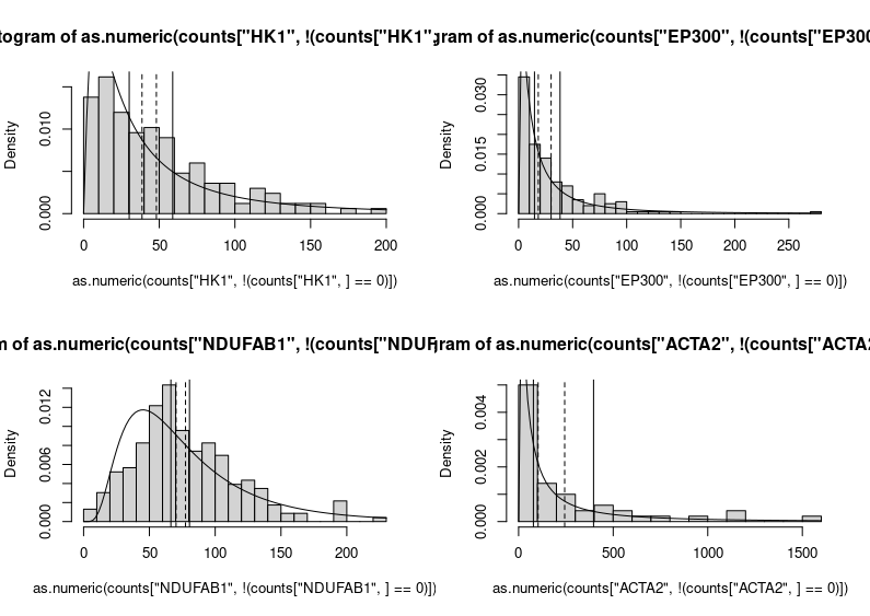
It is not hard to improve our plots, though. We must think about the readers and what we like in other people’s plots. Let’s take the example of a histogram. I’ll use the single cell RNAseq data already presented in my post about medians and means. We want to see if the distribution of gene expressions across many single cells corresponds to a lognormal law. We will plot the expression of four genes, their calculated mean and median, a fitted lognormal distribution and the mean and median of the latter. (NB: We know gene expression does not really follow a lognormal distribution, and comparing distributions is not the proper way to determine if a dataset corresponds to a distribution. If you are interested, have a look at Q-Q plots and the Shapiro-Wilk test.)
Here we go.
Yikes!
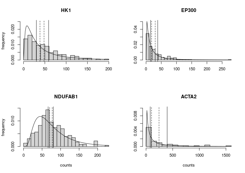
This is horrendous. The fitted distributions are cut, legends are unreadable, and all that grey, so depressing. Let’s improve the figure by choosing different limits for the Y axes to make the entire fitted distributions visible. We can also improve each plot’s title and the labels of the axes. We do not need the latter on each subplot (we can also change the label “density” produced by plotting the fitted distribution into “frequency”, the label we would get by plotting only the histograms. Indeed, the height of the boxes represents the fraction of cells presenting the expression plotted on the X axis.
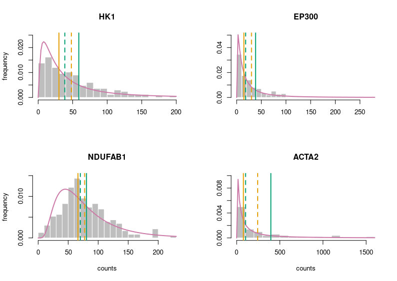
Better. But still very grey. Let’s put some colours on this plot. Those colours are colour-blind-friendly (thanks to the “Colour universal design” of Masataka Okabe and Kei, Ito).
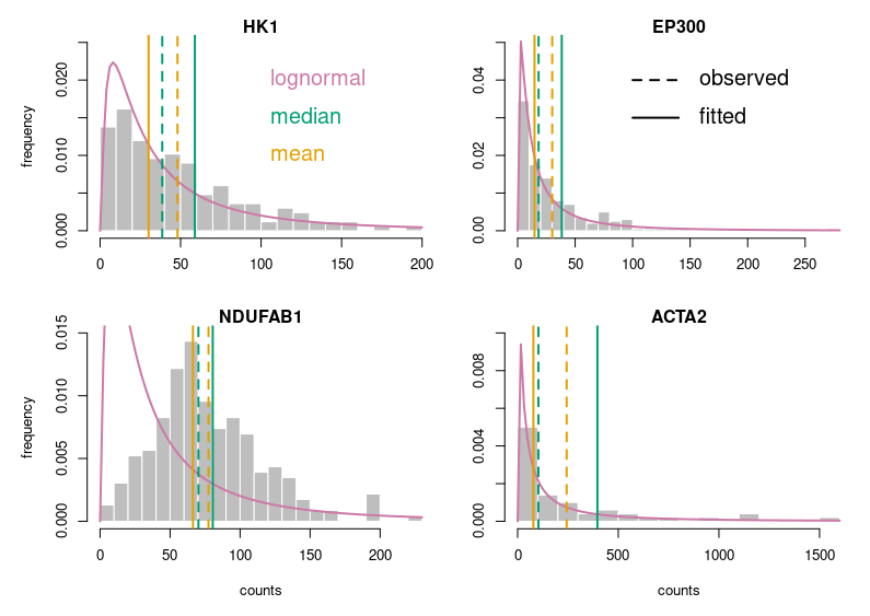
Now, this looks publication-grade. I feel there is still too much white space, so let’s tighten that a bit and add legends.
Of course, for this blog post, I voluntarily started with base R. Using ggplot2 in the first place would have provided a much better starting point. I just wanted to make a point. Here is the code:
# counts is a dataframe with genes in rows and cells in columns

# fitting the counts of hexokinase across all cells to a lognormal law; only consider non-zero values
# (the other four genes are fitted using the same code)
fit_params_HK1 <- fitdistr(as.numeric(counts["HK1",!(counts["HK1",]==0)]),"lognormal")

# to get a 2 by 2 figure without too much empty white space
par(mfrow=c(2,2),
    oma = c(1,1,1,1) + 0.0,
    mar = c(4,4,1,0) + 0.0)

# plot for the hexokinase (the other four genes are plotted using the same code)
# histogram of cell counts
hist(as.numeric(counts["HK1",!(counts["HK1",]==0)]),breaks=20,prob=TRUE,
     col="gray", border = "white",
     main="HK1",xlab=NULL,ylab="frequency",ylim=c(0,0.025))
# lognormal distribution fitted on the counts
curve(dlnorm(x, fit_params_HK1$estimate[1], fit_params_HK1$estimate[2]), col=rgb(204/255,121/255,167/255), lwd=2, add=T)

# observed median and mean
abline(v=median(as.numeric(counts["HK1",!(counts["HK1",]==0)])), col=rgb(0/255,158/255,115/255),lwd=2,lty=2)
abline(v=mean(as.numeric(counts["HK1",!(counts["HK1",]==0)])), col=rgb(230/255,159/255,0/255),lwd=2,lty=2)

# median and mean of the fitted law. remember that the median of a lognormal distributed variable is the mean
# of the log of the variable (meanlog), and its mean is meanlog+sdlog^2/2
abline(v=exp(fit_params_HK1$estimate[1]+(fit_params_HK1$estimate[2])^2/2), col=rgb(0/255,158/255,115/255),lwd=2)
abline(v=exp(fit_params_HK1$estimate[1]), col=rgb(230/255,159/255,0/255),lwd=2)

# plotting the legends for the colours
text(100, 0.02, labels = "lognormal", pos = 4, cex = 1.5, col=rgb(204/255,121/255,167/255))
text(100, 0.015, labels = "median", pos = 4, cex = 1.5, col=rgb(0/255,158/255,115/255))
text(100, 0.01, labels = "mean", pos = 4, cex = 1.5, col=rgb(230/255,159/255,0/255))

# plotting the legend located on the histone acetylase EP300
segments(100,0.04, 140,0.04,col = "black", lty = 2,lwd=2)
segments(100,0.03, 140, 0.03,col = "black", lty = 1,lwd=2)
text(150, 0.04, labels = "observed", pos = 4, cex = 1.5, col="black")
text(150, 0.03, labels = "fitted", pos = 4, cex = 1.5, col="black")
Slides are ubiquitous visual supports for scientific presentations, whether to present results in conferences, report progresses for periodic reviews, or apply to a position or funding. While science is (should be?) paramount, the quality of the slides bears a disproportionate effect on the audience. Here, I will present ten beginner tips – or ten mistakes to avoid – to improve the delivery of your presentation. They aim to improve understanding by making your message clearer, faster, and easier to grasp.
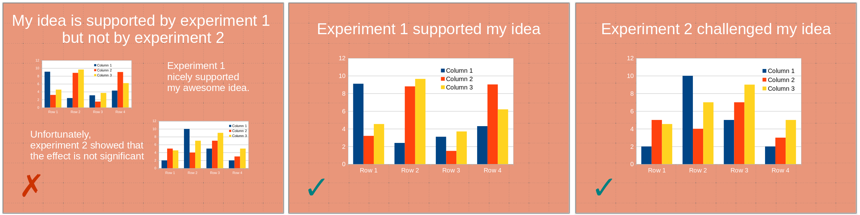
1) One slide should present one point (one idea, one experiment). A slide is not a poster. You might use several panels to illustrate a given point. However, the slide should be entirely dedicated to this one point. A point you are trying to make might be obfuscated by unrelated visuals presenting themselves to the audience’s attention. This might even create confusion if the visuals present related – albeit different –points or experiments, the audience being able to see illustrations that differ from what you are discussing.
2) Avoid slides with only textual content. In particular, except for quotes, do not write down what you are saying. The audience will be torn between listening to you and reading the slide content. Moreover, slightly changing how you express a point might create dissonance, generating confusion.
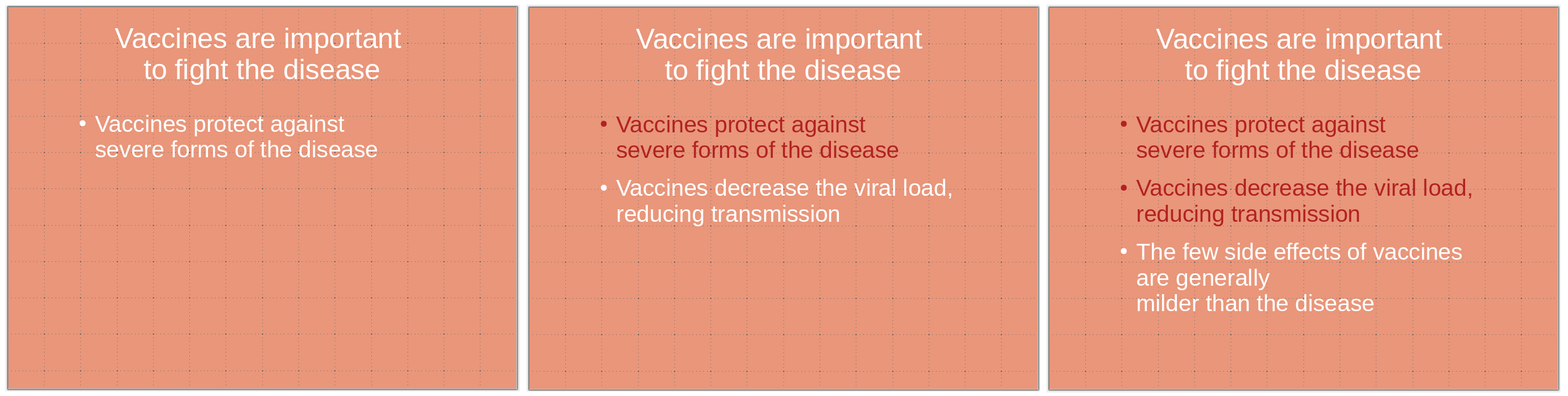
3) Bullet points constitute an exception to the tip above since they can be the sole content of a slide. If you use bullet points, highlight the current point while keeping the previous ones visible. Some people might need time to process them. Depending on the presentation, it can also maintain the logic of the demonstration in everyone’s mind.
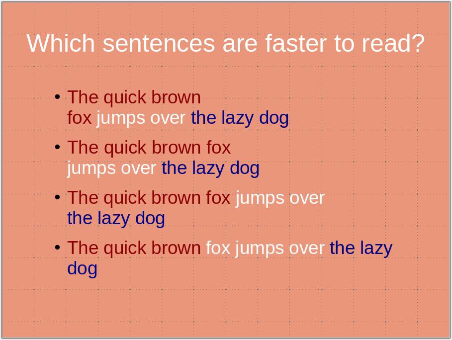
4) Use carriage returns wisely and do not cut expressions or statements. This would slow down the reader, who focuses on the odd break instead of the message. (Also, for the sake of future processing, do not use hard return [new paragraphs ¶] within a sentence or a statement. Use soft returns [line break ↵] instead).
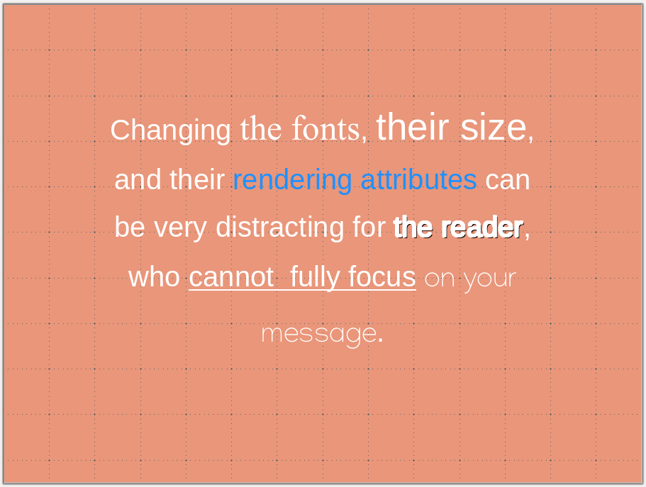
5) Maintain a consistent visual style, including colour codes and fonts. Changing the style distracts the audience. You want all their attention focused on your message rather than following meaningless visual cues. If possible, use the same font size in the same context. If you cannot, it might signal that you have too much text on the slide.
6) Use colour-blind-friendly palettes. About 5% of the population presents some form of colour-blindness, most often red-green. Showing images with green and red fluorescences or a PCA/tSNE/UMAP with red and green points might be a significant strategic error. Not only could your message be lost, but you might also aggravate some audience members (particularly critical in case of a job interview or grant application). There are many resources available providing advice and palettes, such as https://davidmathlogic.com/colorblind https://thenode.biologists.com/data-visualization-with-flying-colors/research/ http://mkweb.bcgsc.ca/colorblind/
Note that changing an image’s hue is perfectly acceptable as it does not alter the signal’s dynamic range or add or remove information. The colours of most biological imaging are artificially added by the acquisition software anyway.
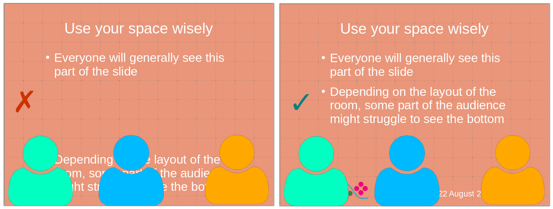
8) Do not put critical information at the bottom of the slide. Depending on the settings of the room where you give the presentation, the bottom of the slide might be hard to see or even masked by the heads of people in the front rows. Use the bottom part of the slide to put logos, date, etc.
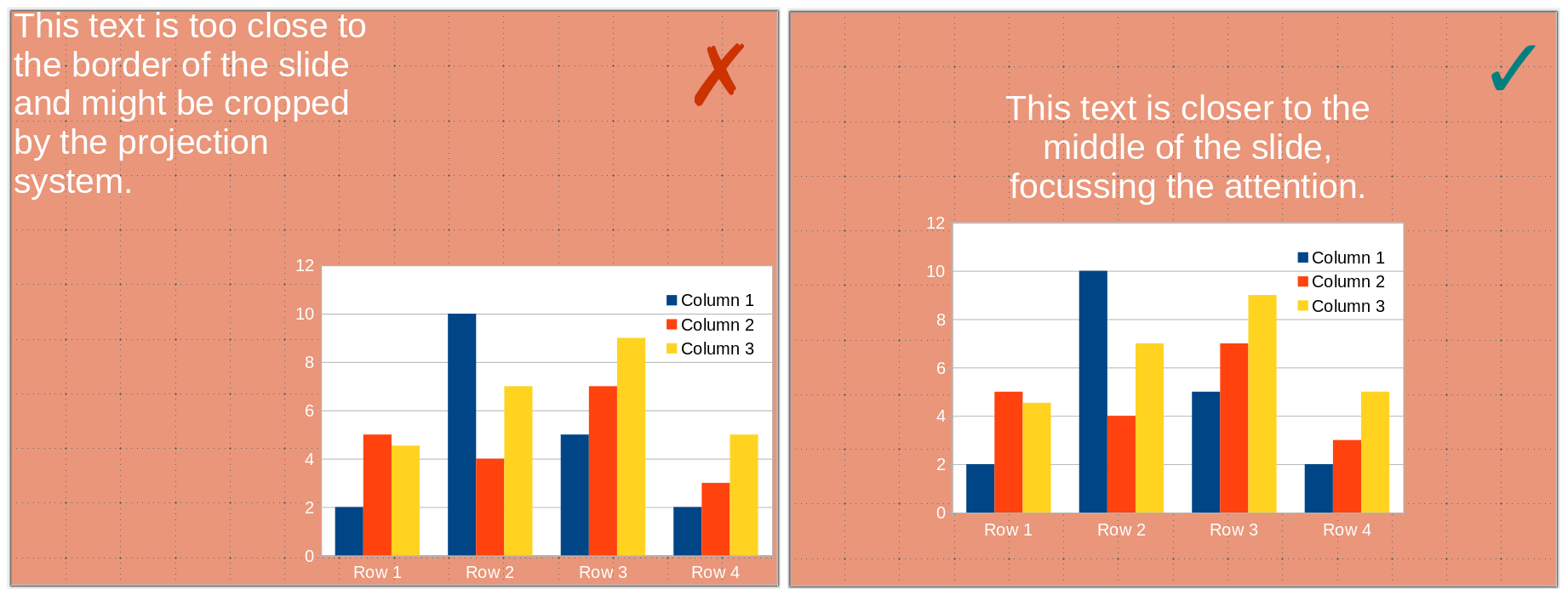
9) Do not put information close to the borders. Some projectors might crop your slides, and you will lose information. Margins also focus the vision, insulating your visual from the surroundings.
10) Finally, and most importantly, proofread, debug, and test your presentation. Test it yourself, trying very hard to be in the position of an audience not knowing its content, and test it with critical friends who are not too familiar with its content but can understand it.
COVID-19 pandemics put mathematical models of biological relevance all over daily newspapers and TV news, raising their profile for the non-scientists. In the life sciences, while mathematical models have always been at the core of some disciplines, such as genetics, they really became mainstream with the rebirth of systems biology a couple of decades ago. However, there are many different modelling approaches, and even specialists often ignore methods they do not use regularly or have not been taught.
After a historical overview, this blog post will then attempt to classify the main types of models used in systems biology according to their principal modalities.
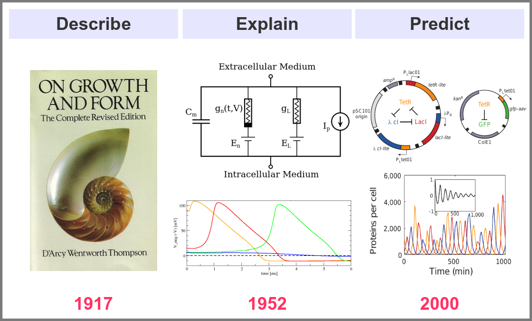
What is the goal of using mathematical models in the life sciences in the first place? Three main aims came out roughly sequentially during the XX century, following the path physics followed over the past two millennia. First, mathematics helps describe the structure and dynamics of living forms and their productions. These models may rely on supposed underlying laws, be purely descriptives, such as the allometric laws. A great example is the famous book “On Growth and Form” by D’Arcy Thompson, attempting to understand living forms based on physical laws.
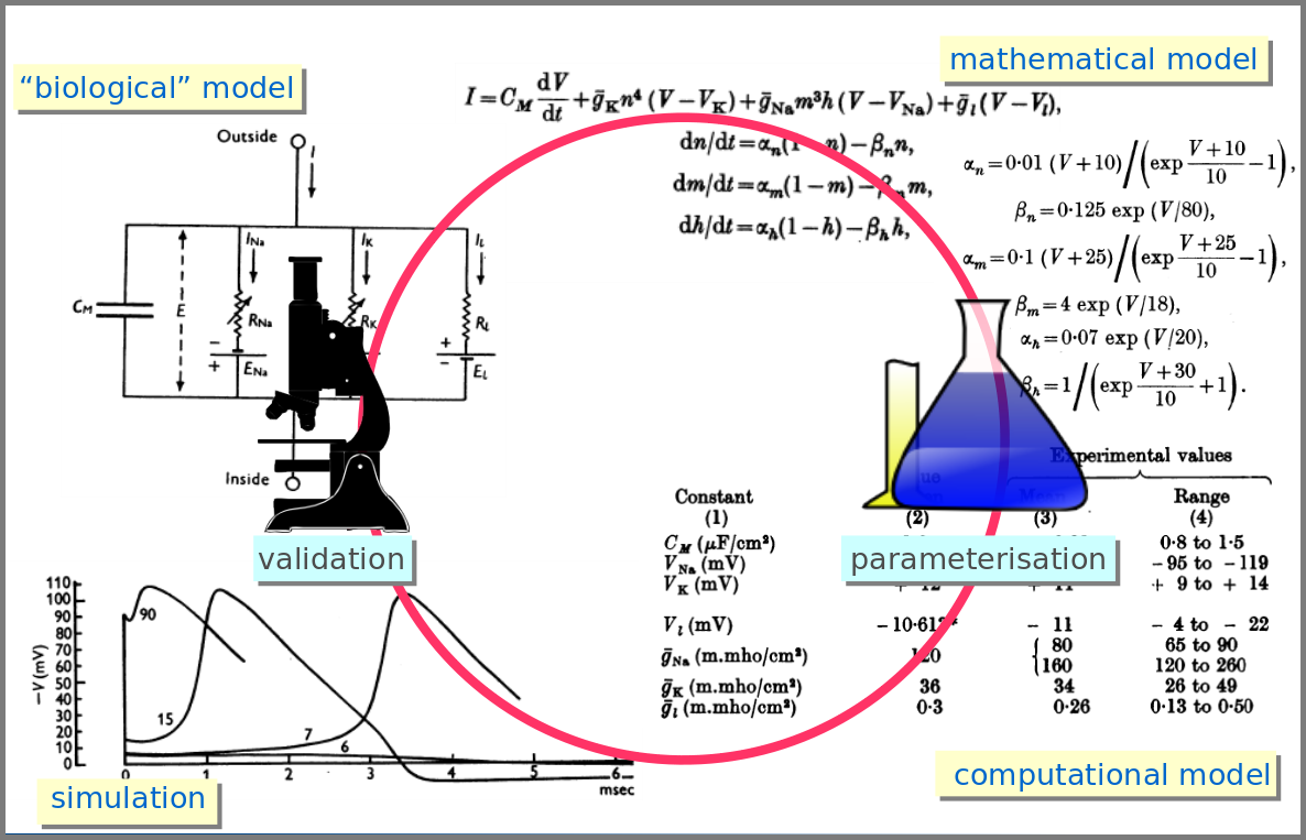
The second aim is to explain the shape and function of living forms. How do the properties of life’s building blocks explain what we can observe? In their masterwork, Alan Hodgkin and Andrew Huxley predicted the existence of ionic channels within the cell membrane and, using a mathematical model, explained how neurons generate action potentials (a work for which they got the Nobel prize).
Finally, can we predict how a system will behave, and can we invent new systems that will behave the way we want them to? This is the purpose of synthetic biology, exemplified in the figure below by the pioneering work of Michael Elowitz and Stanislas Leibler, who built the “repressilator”, a synthetic construct exhibiting sustained oscillations maintained through generations of bacteria.
Obviously, there are no strict boundaries between the three aims, and most models seek to describe, explain, and predict the structures and behaviours of living systems.
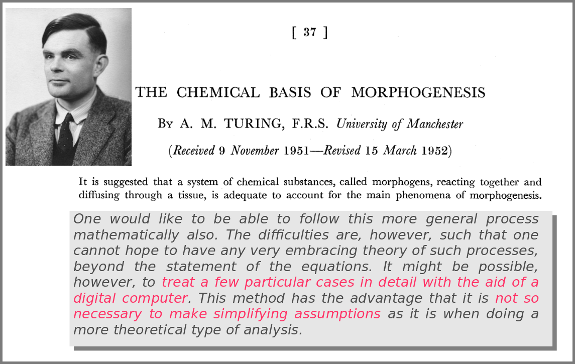
A major shift in the use of mathematical models was the introduction of numerical simulations, made feasible by the invention of computers. The benefits have been laid out by one of the inventors of such computers in an article that indeed contained complex mathematical models but no simulations. In his famous 1952 paper introducing morphogens, Alan Turing suggested that using a digital computer to simulate specific cases of a biological system would allow avoiding the oversimplifications required by analytic solutions.
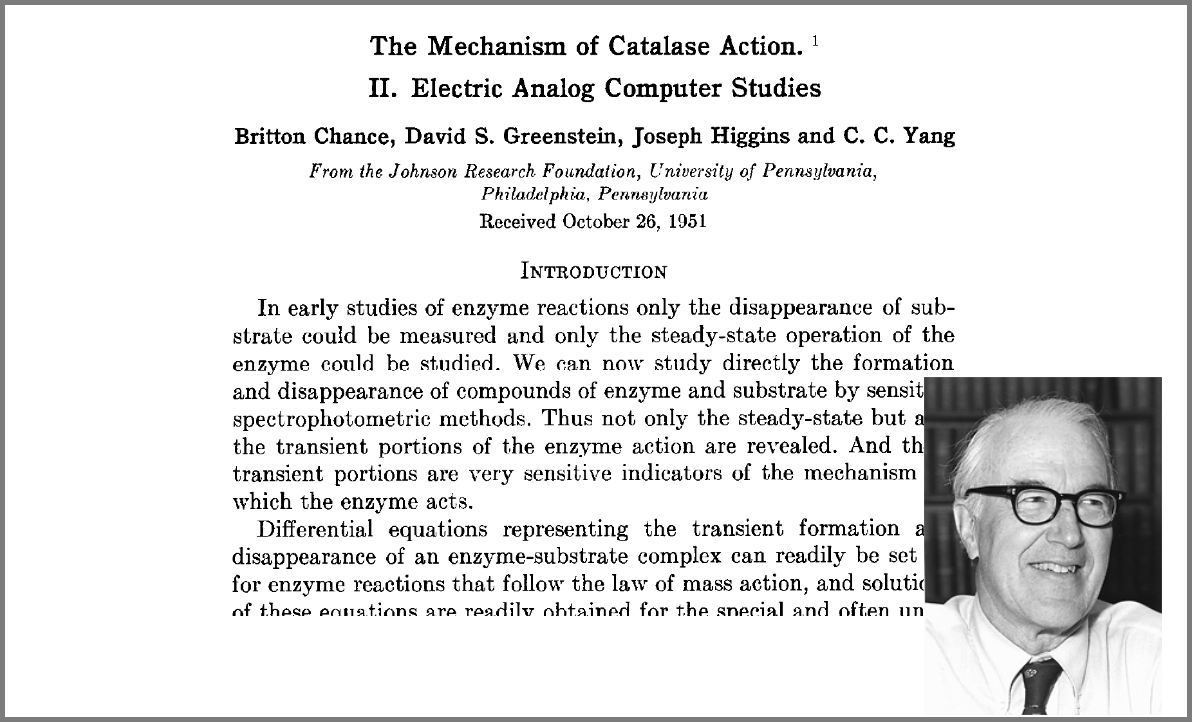
This wish was granted the very same year first by Britton Chance, who built a computer (an analogue one at the time) specifically to solve a differential equation model of a small biochemical pathway.
1952 was also when Hodgkin and Huxley published the action potential model mentioned above, a real Annus Mirabilis for computational modelling in the life sciences.
Before going further, we should ask ourselves, “what is a mathematical model”? According to Wikipedia (as of 4th July 2022), Amathematical model is a description of a system using mathematical concepts and language. I consider that three essential categories of components form mathematical models in systems biology.
Variables represent what we want to know or what we want to compare with the observations. They can characterise a physical entity, e.g., the concentration of a substance, the length of an object or the duration of an event, or be derived from the model itself, for instance, the maximum velocity of an enzymatic reaction.
Relationships mathematically link variables together and represent what we know or what we want to test. They can be static, an affinity constant linked to concentrations or dynamic, such as a rate of change depending on concentrations. Relationships are not necessarily equations. For instance, a sampling might link a variable to a statistical distribution, and logic models use logical statements to attribute values to variables.
Finally, a much-underestimated category is formed by constraints put on the model. Those represent the context of the modelling project or what we consciously decide to ignore. Some constraints are properties of the world, e.g., a concentration must always be positive, the total energy is conserved, and some are properties of the model, such as boundary conditions and objective functions for optimisation procedures. Initial conditions – the values of variables before starting a numerical simulation – are also crucial since a given model might behave differently with different initial conditions, even if neither variables nor relationships are changed.
However, the mathematical model itself is only one brick of a systems biology’s modelling and simulation project as in any natural science domain. Since these models aim to be mechanistic, i.e., anchored in underlying molecular, cellular, tissular, and physiological processes, the first step is to conceptualise a “biological model”. For instance, a biochemical pathway will be a collection of chemical reactions. In the case of Hodgkin and Huxley, who did not know the underlying molecules, the mechanism was based on an electrical analogy, ionic channels being represented by electrical conductances. The “mathematical model” is made up of mathematical relationships linking the variables and constraints. A “computational model”, using the “mathematical model” in conjunction with observed or estimated values, is then simulated. The result is compared with observations, and the loop is iterated.
Now let’s explore the different facets of models used in systems biology, and marvel at their diversity
The variables of a model can represent biological reality at different granularities. In some logical models (often wrongly called Boolean networks), a variable can represent a state, such as presence or absence, 1, 2, 3. Detailed models at the “mesoscopic scale” might represent individual molecules, where a separate variable represents every single particle. Variables can also represent discrete populations of molecules, for instance, the number of molecules of a given chemical class, whose evolution is simulated by stochastic algorithms. In chemical kinetics, the variables whose change is determined using ordinary differential equations often represent continuous concentrations. Finally, some models gloss over the physical parts altogether and use fields to represent what could happen to them.
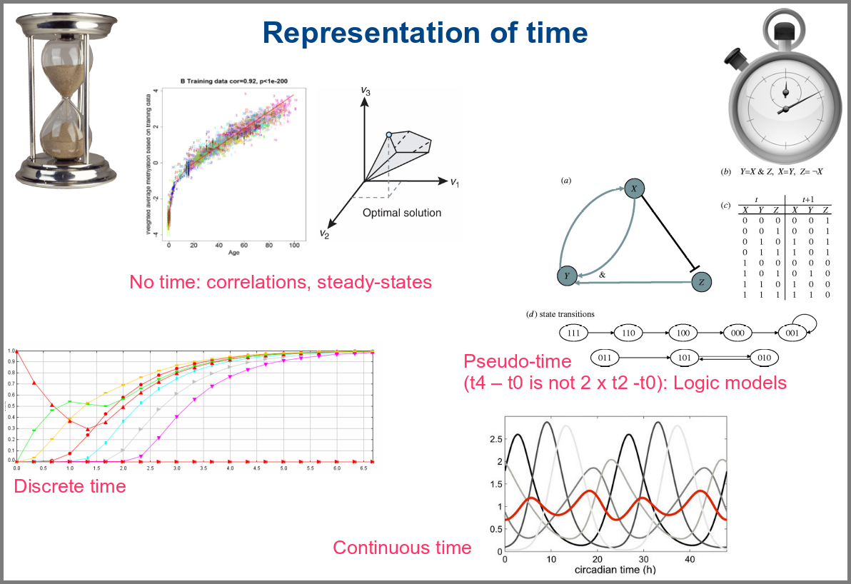
Numerical simulations most often represent the evolution of variable values over “time”. However, the granularity of this “time” may vary. At an extreme, we have models with no representation of time, such as regression models, or implicit representation of time, such as steady-states models. In logical models, as in Petri Net, simulations usually progress along a pseudo-time, where one cannot compare numbers of steps. Time can be discrete, numerical simulations computing a system’s state at fixed intervals, for instance, one second. Finally, models can consider time as continuous, simulations being iterated at various timepoints decided by numerical solvers (note that software might still return results at fixed intervals).
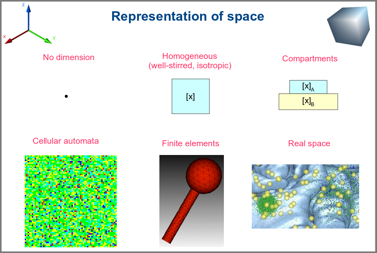
Spacetime being a thing, we also have as many different representations of space. Starting with no space at all, for instance, in noncompartmental analyses of pharmacokinetic models. Space can also be represented by a single homogenous (well-stirred) and isotropic compartment or several of them connected by variables and relationships (multi-compartment models, a.k.a. bathtub models). Cellular automata constitute a particular case, where each compartment is also a model variable whose status depends on its neighbours’. An extension of the multi-compartment modelling represents realistic biological structures using finite elements, each considered homogeneous and isotropic. Finally, space might be represented by continuous variables, where the trajectory of each molecule can be simulated.
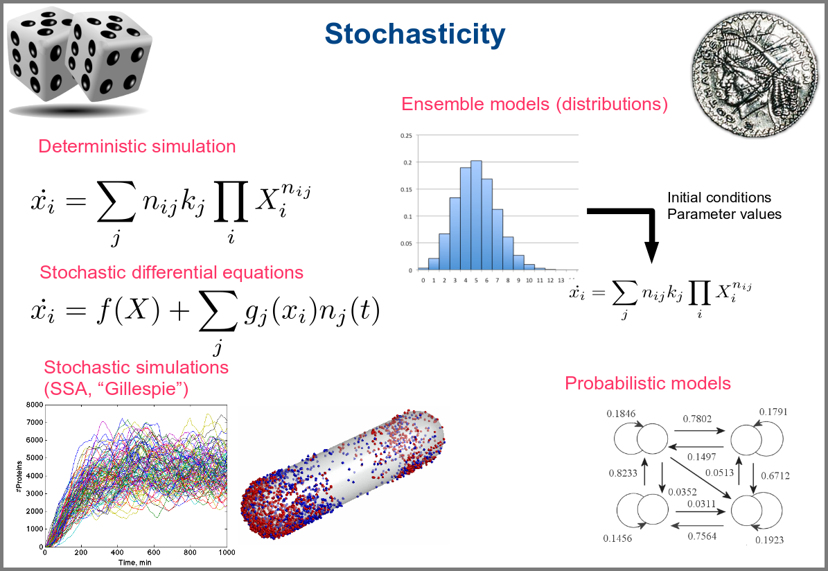
Variability and noise are unavoidable parts of any observation of the natural world, including living systems. Variability can be extrinsic (e.g., due to technical variability), or intrinsic (e.g., actual differences between cells or samples). True noise depends on the size of the system. Taking all those into account in the models can thus be important, and different approaches present different levels and types of stochasticity. As with the other modalities above, stochasticity might be entirely absent, models and simulations being deterministic. One can add different and arbitrary types of noise to simulations with stochastic differential equations. The stochastic aspect might instead emerge directly from the structure of the model, as with the Stochastic Simulation Algorithms (a.k.a. algorithms of the “Gillespie” type). Variability can also be taken into account prior to the simulations, for instance, by sampling initial conditions from distributions, as with ensemble modelling. Finally, in probabilistic models such as Markov models, the entire iteration of the system is based on the probabilities of switching states.
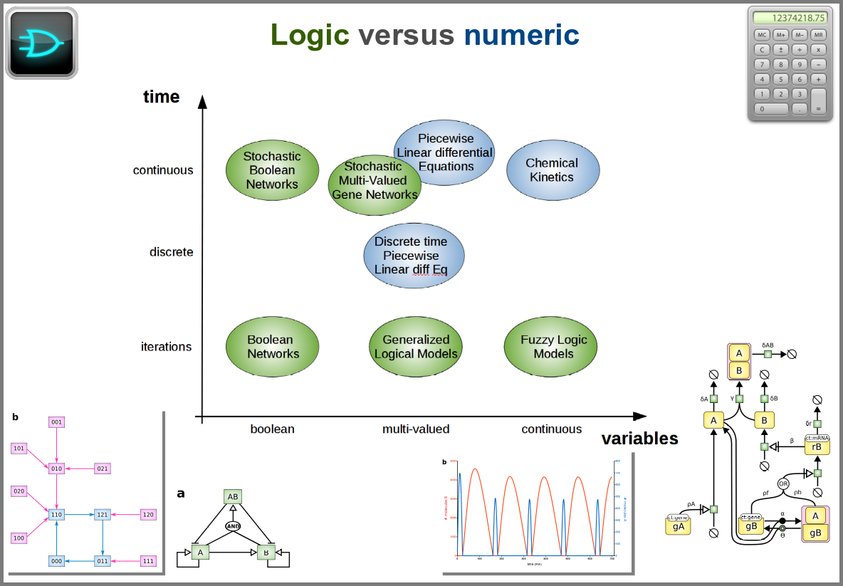
Finally, there are two large families of models based on the type of algorithms used to update the variables. One can compute a variable’s new value by calculating its value either using numerical combinations of previous variables’ values or logic rules taking into account other variable states. Contrary to widespread belief, not all logic models use pseudo-time and Boolean variables. Stochastic Boolean networks can use continuous time, and fuzzy logic models can base their decision on continuous variable values.
Those modalities can be combined in many ways to produce an extremely rich toolkit of modelling approaches. One of the most frequent sources of pain when modelling biological systems is to start with a methodological a priori, often because we are comfortable with an approach, we have the necessary software, or we don’t know better. Doing so can result in under-determined models, endless iterations and failure to get any result. The choice of a modelling approach should be first and foremost based on: 1) the question asked, and 2) the data available to build and validate the model.
References
Chance, B., Greenstein, D. S., Higgins, J. & Yang, C. C. (1952) The mechanism of catalase action. II. Electric analog computer studies. Arch. Biochem. Biophys.37: 322–339. doi:10.1016/0003-9861(52)90195-1
Hodgkin, A.L., Huxley, A.F. (1952). A quantitative description of membrane current and its application to conduction and excitation in nerve. The Journal of Physiology. 117 (4): 500–44. doi:10.1113/jphysiol.1952.sp004764
Stanislas Leibler; Elowitz, Michael B. (2000-01-20). “A synthetic oscillatory network of transcriptional regulators”. Nature403 (6767): 335–338. doi:10.1038/35002125.
Thompson, D. W., 1917. On Growth and Form. Cambridge University Press.
Turing, A. M. (1952). “The chemical basis of morphogenesis”. Philosophical Transactions of the Royal Society of London B. 237 (641): 37–72. doi:10.1098/rstb.1952.0012.
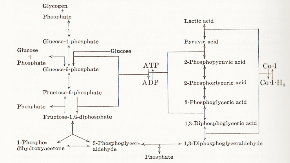
Visual representation of biochemical pathways has been a critical tool for understanding the cellular and molecular systems for a long time. Any knowledge integration project involves a jigsaw puzzle step, where different pieces must be put together. When Feynman cheekily wrote on his blackboard just before his death, “What I cannot create I do not understand”, he meant that he only fully understood a system once he derived a (mathematical) model for it; and interestingly, Feynman is also famous for one of the earliest standard graphical representations of reaction networks, namely the Feynman diagrams to represent models of subatomic particle interactions. The earliest metabolic “map” I possess comes from the 3rd edition of “Outlines of Biochemistry” by Gortner published in 1949. I would be happy to hear if you have older ones.
(I let you find out all the inconsistencies, confusing bits, and error-generating features in this map. This might be food for another text, but I believe this to be a great example to support the creation of standards, best practices, and software tools!)
Until recently, those diagrams were drawn mainly by hand, initially on paper, then using drawing software. There was little thought spent on consistency, visual semantics, or interoperability. This state of affairs changed in the 1990s as part of Systems Biology’s revival. The other thing that changed in the 1990s was the widespread use of computers and software tools to build and analyse models. The child of both trends was the development of standard computer-readable formats to represent biological networks.
When drawing a knowledge representation map, one can divide the decision-making process, and therefore the things we need to encode in order to share the map, into three parts:
What – How can people identify what I represent? A biochemical map is a network built up from nodes linked by arcs. The network may contain only one type of node, for instance, a protein-protein interaction network or an influence network, or be a bipartite graph, like a reaction network – one type of node representing the pools involved in the reactions, the other representing the reactions themselves. One decision is the shape to use for each node so that it carries visual information about the nature of what it represents. Another concerns the arcs linking the nodes, which can also contain visual clues, such as directionality, sign, type of influence, and more. All this must be encoded in some way, either semantically (a code identifying the type of glyphs from an agreed-up list of codes) or graphical (embedding an image or describing the node).
Where – After choosing the glyphs, one needs to place them. The relative position of the information should not always carry much information, but there are some cases where it must, e.g. members of complexes, inclusion in compartments, etc. Furthermore, there is no denying that the relative position of glyphs is also used to convey more subjective information. For instance, a linear chain of reactions induces the idea of a flow, much better than a set of reactions going randomly up and down, right and left. Another unwritten convention is to represent membrane signal transduction on the top of the maps, with the “end-result” – often effect on gene expression – at the bottom, with the idea of a cascading flux of information. The coordinates of the glyphs must then be shared as well.
How – Finally, the impact of a visual representation also depends on aesthetic factors. The relative size of glyphs and labels, the thickness of arcs, the colours, shades and textures, all influence the facility with which viewers absorb the information contained in a map. Relying on such aspects to interpret the meaning of a map should be avoided, particularly if the map is to be shared between different media, where rendering could affect the final aspect. Nevertheless, wanting to keep this aspect as close as possible makes sense.
A bit of history
Different formats have been developed over the years to cover these different aspects with different accuracy and constraints. In order to understand why we have such a variety of description formats on offer, a bit of history might be helpful. Being able to encode the graphical representation of models in SBML was mentioned as early as 2000 (Andrew Finney. Possible Extensions to the Systems Biology Markup Language. 27 November 2000).
In 2002, the group of Hiroaki Kitano presented a graphical editor for the Systems Biology Markup Language (SBML, Hucka et al 2003, Keating et al 2020), called SBedit, and proposed extensions to SBML necessary for encoding maps (Tanimura et al. Proposal for SBEdit’s extension of SBML-Level-1. 8 July 2002). This software later became CellDesigner (Funahashi et al 2003), a full-featured modelling developing environment using SBML as its native format. All graphical information is encoded in CellDesigner-specific annotations using the SBML extension system. In addition to the layout (the where), CellDesigner proposed a set of standardised glyphs to use for representing different types of molecular entities and different relationships (the what) (Kitano et al 2003). At the same time, Herbert Sauro developed an extension to SBML to encode the maps designed in the software JDesigner (Herbert Sauro. JDesigner SBMLAnnotation. 8 January 2003). Both CellDesigner and JDesigner annotations could also encode the appearance of glyphs (the how).
Once the SBML Layout annotations were finalised, the SBML and BioPAX communities came together to standardise visual representations for biochemical pathways. This led to the Systems Biology Graphical Notation, a set of three standard graphical languages with agreed-upon symbols and rules to assemble them (the what, Le Novère et al 2009). While the shape of SBGN glyphs determines their meaning, neither their placement in the map nor their graphical attributes (colour, texture, edge thickness, the how) affect the map semantics. SBGN maps are ultimately images and can be exchanged as such, either in bitmaps or vector graphics. They are also graphs and can be exchanged using graph formats like GraphML. However, sharing and editing SBGN maps would be much easier if more semantics were encoded than graphical details. This feeling led to the development of SBGN-ML (van Iersel et al 2012), which encodes not only the SBGN part of SBGN maps but also the layout and size of graph elements.
So we have at least three solutions to encode biochemical maps using XML standards from the COMBINE community (Hucka et al 2015):
1) SBGN-ML,
2) SBML with Layout extension (controlled Layout annotations in Level 2 and Layout package in Level 3), and
3) SBML with proprietary extensions.
Regarding the latter, we will only consider the CellDesigner variant for two reasons. Firstly, CellDesigner is the most used graphical model designer in systems biology (at the time of writing, the articles describing the software have been cited over 1000 times). Secondly, CellDesigner’s SBML extensions are used in other software tools. These three solutions are not equivalent; they present different advantages and disadvantages, and round-tripping is generally impossible.
SBGN-ML
Curiously, despite its name, SBGN-ML does not explicitly describe the SBGN part of the maps (the what). Since the shape of nodes is a standard, it is only necessary to mention their type, and any supporting software will know which symbol to use. For instance, SBGN-ML will not specify that a protein X must be represented with a round-corner rectangle. It will only say that there is a macromolecule X at a particular position with given width and height. Any SBGN-supporting software must know that a round-corner rectangle represents a macromolecule. The consequence is that SBGN-ML cannot be used to encode maps using non-SBGN symbols. However, software tools can decide to use different symbols attributed to a given class of SBGN objects while rendering the maps. For example, instead of using a round-corner rectangle each time a glyph’s class is macromolecule, it could use a star. The resulting image would not be an SBGN map. However, if modified and saved back in SBGN-ML, it could be recognised by another supporting software. Such behaviour is not to be encouraged if we want people to get used to SBGN symbols, but it provides a certain level of interoperability.
What SBGN-ML explicitly describes instead are the parts that SBGN itself does not regulate but are specific to the map. That includes the size of the glyphs (bounding box), the textual labels, as well as the positions of glyphs (the where). SBGN-ML currently does not encode rendering properties such as text size, colours and textures (the how). However, the language provides an element extension, analogous to the SBML annotation, that allows augmenting the language. One can use this element to extend each glyph or encode style, and the community started to do so in an agreed-upon manner.
Note that SBGN-ML only encodes the graph. While it contains a certain amount of biological semantics – linked to the identity of the glyphs – it is not a general-purpose format that would encode advanced semantics of regulatory features such as BioPAX (Demir et al. 2010), or mathematical relationships such as SBML. However, users can distribute SBML files along with SBGN-ML files, for instance, in a COMBINE Archive (Bergmann et al 2014). Unfortunately, there is currently no blessed way to map an SBML element, such as a particular species, to a given SBGN-ML glyph.
SBML Level 3 + Layout and Render packages
As we mentioned before, SBML Level 3 provides two packages helping with the visual representations of networks: Layout (the where) and Render (the how). Contrarily to SBGN-ML, which is meant to describe maps in a standard graphical notation, the SBML Level 3 packages do not restrict the way one represents biochemical networks. This provides more flexibility to the user but decreases the “stand-alone” semantics content of the representations. I.e. if non-standard symbols are used, their meaning must be defined in an external legend. It is, of course, possible to use only SBGN glyphs to encode maps. The visual rendering of such a file will be SBGN, but the automatic analysis of the underlying format will be more challenging.
The SBML Layout package permits encoding the position of objects, points, curves and bounding boxes. Curves can have complex shapes encoded as Béziers curves. The package allows distinguishing between different general types of nodes such as compartments, molecular species, reactions and text. However, there is little biological semantics encoded by the shapes, either regarding the nodes (e.g. nothing distinguishes a simple chemical from a protein) or the edges (one cannot distinguish an inhibition from a stimulation). In addition, the SBML Render package permits to define styles that can be applied to types of glyphs. This includes colours and gradients, geometric shapes, properties of text, lines, line-endings etc. Render can encode a wide variety of graphical properties, and pave the gap to generic graphical formats such as SVG.
If we are trying to visualise a model, one advantage of using SBML packages is that all the information is included in a single file, providing a straightforward mapping between the model constructs and their representation. This goes a long way to solve the issue of the biological semantics mentioned above since it can be retrieved from the SBML Core elements linked to the Layout elements. Let us note that while SBML Layout+Render do not encode the nature of the objects represented by the glyphs (the what) using specific structures, this can be retrieved via the attributes sboTerm of the corresponding SBML Core elements, using the appropriate values from the Systems Biology Ontology (Courtot et al 2011).
CellDesigner notation
CellDesigner uses SBML (currently Level 2) as its native language. However, it extended it with its own proprietary annotation, keeping the SBML perfectly valid (which is also the way software tools such as JDesigner operate). Visually, the CellDesigner notation is close to SBGN Process Descriptions, having been the strongest inspiration for the community effort. CellDesigner offers an SBGN-View mode, that produces graphs closer to pure SBGN PD.
CellDesigner’s SBML extensions increase the semantics of SBML elements such as molecular species or regulatory arcs in a way not dissimilar to SBGN-ML. In addition, it provides a description of each glyph linked to the SBML elements, covering the ground of SBML Layout and Render. The SBML extensions being specific to CellDesigner, they do not offer the flexibility of SBML Render. However, the limited spectrum of possibilities might make the support easier.
CellDesigner notation
SBML Layout+Render
SBGN-ML
Encodes the what
✓
✓
✓
Encodes the where
✓
✓
✓
Encodes the how
✓
✓
✓
Contains the mathematical model part
✓
✓
✗
Writing supported by more than 1 tool
✗
✓
✓
Reading supported by more than 1 tool
✓
✓
✓
Is a community standard
✗
✓
✓
Examples of usages and conversions
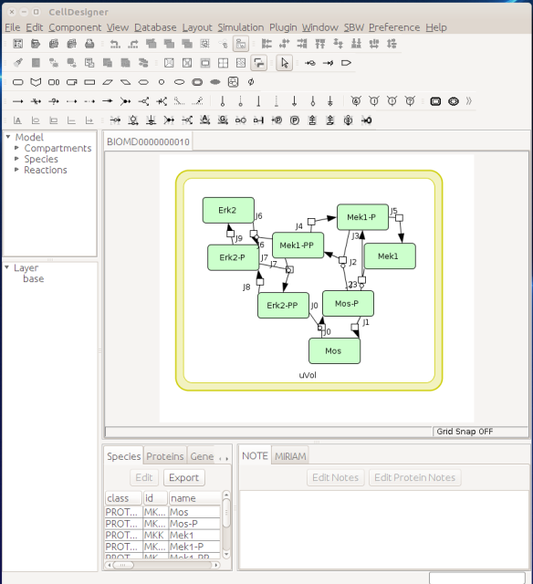
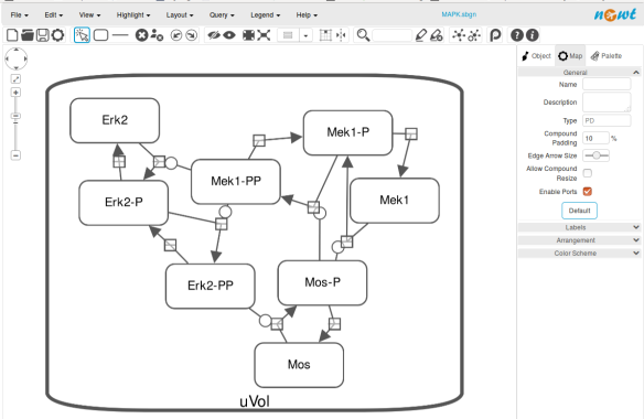
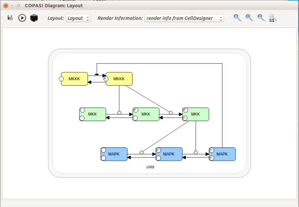
Now let us see the three formats in action. We start with SBGN-ML. First, we can load a model – for instance from BioModels (Chelliah et al 2015 ) – in CellDesigner (version 4.4 at the time of writing). Here we will use the model BIOMD0000000010, an SBML version of the MAP kinase model described in Kholodenko et al (2000).
From an SBML file that does not contain any visual representation, CellDesigner created one using its auto-layout functions. One can then export an SBGN-ML file. This SBGN-ML file can be imported, for instance, in Cytoscape (Shannon et al. 2003) 2.8 using the CySBGN plugin (Gonçalves et al 2013).
The position and size of nodes are conserved, but edges have different sizes (and the catalysis glyph is wrong). The same SBGN-ML file can be open in the online SBGN editor Newt.
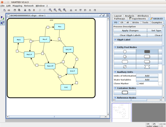
An alternative to CellDesigner to produce the SBGN-ML map could be Vanted (Junker et al 2006, version 2.6.4 at the time of writing). Using the same model from BioModels, we can auto-layout the map (we used the organic layout here) and then convert the graph to SBGN using the SBGN-ED plugin (Czauderna et al 2010).
The map can then be saved as SBGN-ML and as before, opened in Newt.
The positions of the nodes are conserved. However, the connection of edges is a bit different. In that case, Newt is slightly more SBGN compliant.
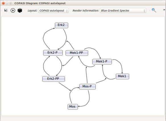
Then, let us start with a vanilla SBML file. We can import our BIOMD0000000010 model in COPASI (Hoops et al 2006, version 4.22 at the time of writing). COPASI now offers auto-layout capabilities, with the possibility of manually editing the resulting maps.
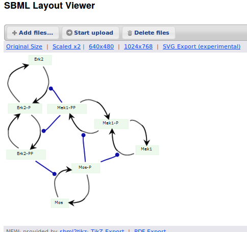
When we export the model in SBML, it will now contain the map encoded with the Layout and Render packages. When the model is uploaded in any software tool supporting the packages, we will retrieve the map. For instance, we can use the SBML Layout Viewer. Note that if the layout is conserved, it is not the case with the rendering.
Alternatively, we can load the model to CellDesigner, and manually generate a nice map (NB: a CellDesigner plugin that can read SBML Layout was implemented during Google Summer of Code 2014 . It is part of the JSBML project).
We can create an SBML Layout using the CellDesigner layout converter. Then, when we import the model in COPASI, we can visualise the map encoded in Layout. NB: here, the difference in appearance is due to a problem in the CellDesigner converter, not COPASI.
The same model can be loaded in the SBML Layout Viewer.
How do I choose between the formats?
There is, unfortunately, no unique solution at the moment. The main question one has to ask is what do we want to do with the visual maps?
Are they meant to be a visual representation of an underlying model, the model being the critical part that needs to be exchanged? If that is the case, SBML packages or CellDesigner notation should be used.
Does the project mostly/only involves graphical representations, and those must be exchanged? CellDesigner or SBGN-ML would therefore be better.
Does the rendering of graphical elements matter? In that case, SBML packages or CellDesigner notations are currently better (but that is going to change soon).
Is standardisation important for the project, in addition to immediate interoperability? If yes, SBML packages or SBGN-ML would be the way to go.
All those questions and more have to be clearly spelt out at the beginning of a project. The answer will quickly emerge from the answers.
Acknowledgements
Thanks to Frank Bergmann, Andreas Dräger, Akira Funahashi, Sarah Keating, Herbert Sauro for help and corrections.
References
Bergmann FT, Adams R, Moodie S, Cooper J, Glont M, Golebiewski M, Hucka M, Laibe C, Miller AK, Nickerson DP, Olivier BG, Rodriguez N, Sauro HM, Scharm M, Soiland-Reyes S, Waltemath D, Yvon F, Le Novère N (2015) COMBINE archive and OMEX format: one file to share all information to reproduce a modeling project. BMC Syst Biol 15, 369. doi:10.1186/s12859-014-0369-z
Chelliah V, Juty N, Ajmera I, Raza A, Dumousseau M, Glont M, Hucka M, Jalowicki G, Keating S, Knight-Schrijver V, Lloret-Villas A, Natarajan K, Pettit J-B, Rodriguez N, Schubert M, Wimalaratne S, Zhou Y, Hermjakob H, Le Novère N, Laibe C (2015) BioModels: ten year anniversary. Nucleic Acids Res 43(D1), D542-D548. doi:10.1093/nar/gku1181
Courtot M, Juty N, Knüpfer C, Waltemath D, Zhukova A, Dräger A, Dumontier M, Finney A, Golebiewski M, Hastings J, Hoops S, Keating S, Kell DB, Kerrien S, Lawson J, Lister A, Lu J, Machne R, Mendes P, Pocock M, Rodriguez N, Villeger A, Wilkinson DJ, Wimalaratne S, Laibe C, Hucka M, Le Novère N. Controlled vocabularies and semantics in Systems Biology. Mol Syst Biol 7, 543. doi:10.1038/msb.2011.77
Czauderna T, Klukas C, Schreiber F (2010) Editing, validating and translating of SBGN maps. Bioinformatics 26(18), 2340-2341. doi:10.1093/bioinformatics/btq407
Demir E, Cary MP, Paley S, Fukuda K, Lemer C, Vastrik I, Wu G, D’Eustachio P, Schaefer C, Luciano J, Schacherer F, Martinez-Flores I, Hu Z, Jimenez-Jacinto V, Joshi-Tope G, Kandasamy K, Lopez-Fuentes AC, Mi H, Pichler E, Rodchenkov I, Splendiani A, Tkachev S, Zucker J, Gopinathrao G, Rajasimha H, Ramakrishnan R, Shah I, Syed M, Anwar N, Babur O, Blinov M, Brauner E, Corwin D, Donaldson S, Gibbons F, Goldberg R, Hornbeck P, Luna A, Murray-Rust P, Neumann E, Ruebenacker O, Samwald M, van Iersel M, Wimalaratne S, Allen K, Braun B, Carrillo M, Cheung KH, Dahlquist K, Finney A, Gillespie M, Glass E, Gong L, Haw R, Honig M, Hubaut O, Kane D, Krupa S, Kutmon M, Leonard J, Marks D, Merberg D, Petri V, Pico A, Ravenscroft D, Ren L, Shah N, Sunshine M, Tang R, Whaley R, Letovksy S, Buetow KH, Rzhetsky A, Schachter V, Sobral BS, Dogrusoz U, McWeeney S, Aladjem M, Birney E, Collado-Vides J, Goto S, Hucka M, Le Novère N, Maltsev N, Pandey A, Thomas P, Wingender E, Karp PD, Sander C, Bader GD (2010) The BioPAX Community Standard for Pathway Data Sharing. Nat Biotechnol, 28, 935–942. doi:10.1038/nbt.1666
Funahashi A, Morohashi M, Kitano H, Tanimura N (2003) CellDesigner: a process diagram editor for gene-regulatory and biochemical networks. Biosilico 1 (5), 159-162
Gauges R, Rost U, Sahle S, Wegner K (2006) A model diagram layout extension for SBML. Bioinformatics 22(15), 1879-1885. doi:10.1093/bioinformatics/btl195
Gauges R, Rost U, Sahle S, Wengler K, Bergmann FT (2015) The Systems Biology Markup Language (SBML) Level 3 Package: Layout, Version 1 Core. J Integr Bioinform 12(2), 267. doi:10.2390/biecoll-jib-2015-267
Gonçalves E, van Iersel M, Saez-Rodriguez J (2013) CySBGN: A Cytoscape plug-in to integrate SBGN maps. BMC Bioinfo 14, 17. doi:10.1186/1471-2105-14-17
Hoops S, Sahle S, Gauges R, Lee C, Pahle J, Simus N, Singhal M, Xu L, Mendes P, Kummer U (2006) COPASI-a COmplex PAthway SImulator. Bioinformatics 22(24), 3067-3074. doi:10.1093/bioinformatics/btl485
Hucka M, Bolouri H, Finney A, Sauro HM, Doyle JC, Kitano H, Arkin AP, Bornstein BJ, Bray D, Cornish-Bowden A, Cuellar AA, Dronov S, Ginkel M, Gor V, Goryanin II, Hedley WJ, Hodgman TC, Hunter PJ, Juty NS, Kasberger JL, Kremling A, Kummer U, Le Novère N, Loew LM, Lucio D, Mendes P, Mjolsness ED, Nakayama Y, Nelson MR, Nielsen PF, Sakurada T, Schaff JC, Shapiro BE, Shimizu TS, Spence HD, Stelling J, Takahashi K, Tomita M, Wagner J, Wang J (2003) The Systems Biology Markup Language (SBML): A Medium for Representation and Exchange of Biochemical Network Models. Bioinformatics, 19, 524-531. doi:10.1093/bioinformatics/btg015
Hucka M, Nickerson DP, Bader G, Bergmann FT, Cooper J, Demir E, Garny A, Golebiewski M, Myers CJ, Schreiber F, Waltemath D, Le Novère N (2015) Promoting coordinated development of community-based information standards for modeling in biology: the COMBINE initiative. Frontiers Bioeng Biotechnol 3, 19. doi:10.3389/fbioe.2015.00019
Junker BH, Klukas C, Schreiber F (2006) VANTED: A system for advanced data analysis and visualization in the context of biological networks. BMC Bioinfo 7, 109. doi:10.1186/1471-2105-7-109
Sarah M Keating, Dagmar Waltemath, Matthias König, Fengkai Zhang, Andreas Dräger, Claudine Chaouiya, Frank T Bergmann, Andrew Finney, Colin S Gillespie, Tomáš Helikar, Stefan Hoops, Rahuman S Malik-Sheriff, Stuart L Moodie, Ion I Moraru, Chris J Myers, Aurélien Naldi, Brett G Olivier, Sven Sahle, James C Schaff, Lucian P Smith, Maciej J Swat,Denis Thieffry, Leandro Watanabe, Darren J Wilkinson, Michael L Blinov, Kimberly Begley, James R Faeder, Harold F Gómez, Thomas M Hamm, Yuichiro Inagaki, Wolfram Liebermeister, Allyson L Lister, Daniel Lucio, Eric Mjolsness, Carole J Proctor, Karthik Raman, Nicolas Rodriguez, Clifford A Shaffer, Bruce E Shapiro, Joerg Stelling, Neil Swainston, Naoki Tanimura, John Wagner, Martin Meier-Schellersheim, Herbert M Sauro, Bernhard Palsson, Hamid Bolouri, Hiroaki Kitano, Akira Funahashi, Henning Hermjakob, John C Doyle, Michael Hucka, and the SBML Level3Community members: Richard R Adams,Nicholas A Allen,Bastian R Angermann,Marco Antoniotti,Gary D Bader,Jan Červený,Mélanie Courtot,Chris D Cox,Piero Dalle Pezze,Emek Demir,William S Denney,Harish Dharuri,Julien Dorier,Dirk Drasdo,Ali Ebrahim,Johannes Eichner,Johan Elf,Lukas Endler,Chris T Evelo,Christoph Flamm,Ronan MT Fleming,Martina Fröhlich,Mihai Glont,Emanuel Gonçalves,Martin Golebiewski,Hovakim Grabski,Alex Gutteridge,Damon Hachmeister,Leonard A Harris,Benjamin D Heavner,Ron Henkel,William S Hlavacek,Bin Hu,Daniel R Hyduke,Hidde Jong,Nick Juty,Peter D Karp,Jonathan R Karr,Douglas B Kell,Roland Keller,Ilya Kiselev,Steffen Klamt,Edda Klipp,Christian Knüpfer,Fedor Kolpakov,Falko Krause,Martina Kutmon,Camille Laibe,Conor Lawless,Lu Li,Leslie M Loew,Rainer Machne,Yukiko Matsuoka,Pedro Mendes,Huaiyu Mi,Florian Mittag,Pedro T Monteiro,Kedar Nath Natarajan,Poul MF Nielsen,Tramy Nguyen,Alida Palmisano,Jean-Baptiste Pettit,Thomas Pfau,Robert D Phair,Tomas Radivoyevitch,Johann M Rohwer,Oliver A Ruebenacker,Julio Saez-Rodriguez,Martin Scharm,Henning Schmidt,Falk Schreiber,Michael Schubert,Roman Schulte,Stuart C Sealfon,Kieran Smallbone,Sylvain Soliman,Melanie I Stefan,Devin P Sullivan,Koichi Takahashi,Bas Teusink,David Tolnay,Ibrahim Vazirabad,Axel Kamp,Ulrike Wittig,Clemens Wrzodek,Finja Wrzodek,Ioannis Xenarios,Anna Zhukova andJeremy Zucker (2020) SBML Level 3: an extensible format for the exchange and reuse of biological models. Mol Syst Biol 16, e9110. doi:10.15252/msb.20199110
Kholodenko BN (2000) Negative feedback and ultrasensitivity can bring about oscillations in the mitogen-activated protein kinase cascades. Eur J Biochem.267(6), 1583-1588. doi:10.1046/j.1432-1327.2000.01197.x
Le Novère N, Hucka M, Mi H, Moodie S, Shreiber F, Sorokin A, Demir E, Wegner K, Aladjem M, Wimalaratne S, Bergman FT, Gauges R, Ghazal P, Kawaji H, Li L, Matsuoka Y, Villéger A, Boyd SE, Calzone L, Courtot M, Dogrusoz U, Freeman T, Funahashi A, Ghosh S, Jouraku A, Kim S, Kolpakov F, Luna A, Sahle S, Schmidt E, Watterson S, Goryanin I, Kell DB, Sander C, Sauro H, Snoep JL, Kohn K, Kitano H (2009) The Systems Biology Graphical Notation. Nat Biotechnol 27, 735-741. doi:10.1038/nbt.1558
Shannon P, Markiel A, Ozier O, Baliga NS, Wang JT, Ramge D, Amin N, Schwikowski B, Ideker T (2003) Cytoscape: a software environment for integrated models of biomolecular interaction networks. Bioinformatics 13, 2498-2504. doi:10.1101/gr.1239303
van Iersel MP, Villéger AC, Czauderna T, Boyd SE, Bergmann FT, Luna A, Demir E, Sorokin A, Dogrusoz U, Matsuoka Y, Funahashi A, Aladjem MI, Mi H, Moodie SL, Kitano H, Le Novère N, Schreiber F (2012) Software support for SBGN maps: SBGN-ML and LibSBGN. Bioinformatics 28, 2016-2021. doi:10.1093/bioinformatics/bts270
Quelle ponctuation utiliser dans les listes à puces ou numérotées ? Si l’on essaie de comprendre les règles en accumulant les exemples, le découragement vient rapidement, car il semble que le hasard règne en maître. Si l’on trouve une liste de ces règles, le soulagement est de courte durée tant celles-ci semblent arbitraires et les exceptions nombreuses. Je vais proposer à la fin de ce billet un algorithme graphique en deux parties, pour vous aider à choisir la casse des premières lettres des éléments de liste et la ponctuation à la fin de chaque élément. Mais avant, ça je vais fusionner toutes les règles en une seule, et présenter des exemples vous aidant à la comprendre.
Avertissement : ce billet ne concerne que les listes insérées dans des textes. S’il s’agit de listes insérées dans des diapositives de présentations, la rapidité de lecture et la facilité de mise en page doit être prise en compte, et on préférera souvent commencer chaque élément par une majuscule et omettre la ponctuation à la fin de celui-ci.
Revenons à cette fameuse unique Règle pour les Gouverner Toutes ; quelle est-elle ? C’est tout simple :
Si on supprime le formatage de la liste, à savoir, passages à la ligne et puces, la ponctuation du texte résultant doit rester correcte.
Prenons une liste simple.
Le cerveau comporte trois grandes parties : –le prosencéphale ; –le mésencéphale ; –le rhombencéphale.
Si l’on supprime le formatage de la liste ci-dessus, on obtient :
Le cerveau comporte trois grandes parties : le prosencéphale ;le mésencéphale ;le rhombencéphale.
La ponctuation de cette phrase est tout à fait correcte puisqu’elle commence par une majuscule, ne contient pas de majuscules au milieu, suivant les deux-points et les point-virgules, et se termine par un point.
Aparté : le tiret commençant l’entrée d’une liste est un tiret semi-cadratin « – ». Ce n’est ni un trait d’union « - », ni un tiret cadratin « — », ni bien sûr le symbole mathématique moins « − ». Ce tiret est suivi d’une espace insécable, comme il l’est quand il précède une incise. Fin de l’aparté.
On ferme chaque élément par une ponctuation non fermante, sauf le dernier. On aurait pu remplacer les point-virgules par des virgules. Dans ce cas, on aurait également pu ajouter la conjonction de coordination « et » après le pénultième élément (après la virgule !).
Le cerveau comporte trois grandes parties : – le prosencéphale, – le mésencéphale, et – le rhombencéphale.
L’absence de ponctuation à la fin de chaque élément, comme l’utilisation d’un point rend la ponctuation incorrecte :
Le cerveau comporte trois grandes parties : le prosencéphale le mésencéphale le rhombencéphale
Le cerveau comporte trois grandes parties : le prosencéphale.le mésencéphale.le rhombencéphale.
Ce serait également le cas si nous avions commencé chaque élément par une majuscule.
Le cerveau comporte trois grandes parties : Le prosencéphale ;Le mésencéphale ;Le rhombencéphale.
Dans la liste précédente, les éléments ne sont pas indépendants de la phrase d’entrée. Ce n’est parfois pas le cas, par exemple si cette dernière est du type « Remarques : » ou « À noter : » (mais pas « À noter que : »). Dans ces cas-là, les éléments de la liste sont des phrases complètes, indépendantes non seulement de la phrase d’entrée, mais également l’une de l’autre. Elles sont ponctuées en conséquence.
Remarques : – Le prosencéphale contient la vaste majorité des neurones du cerveau des êtres humains. – Le mésencéphale est atteint dans la maladie de Parkinson. – Le rhombencéphale contrôle les fonctions vitales et autonomes.
Remarques : Le prosencéphale contient la vaste majorité des neurones du cerveau des êtres humains.Le mésencéphale est atteint dans la maladie de Parkinson.Le rhombencéphale contrôle les fonctions vitales et autonomes.
Les listes ci-dessus étaient précédées d’une phrase ouverte, se terminant par deux-points. Cela aurait également été le cas si elle s’était terminée par un point-virgule ou une virgule (voir plus bas le cas des listes emboîtées). Si la phrase d’entrée est fermée, c’est-à-dire qu’elle se termine par un point, un point d’exclamation ou un point d’interrogation, les règles sont différentes, car les éléments sont eux-mêmes des phrases.
Laquelle des informations suivantes est erronée ? – Le prosencéphale est la partie la plus antérieure du cerveau. – Le mésencéphale est atteint dans le diabète sucré. – Le rhombencéphale contrôle les fonctions vitales et autonomes.
Laquelle des informations suivantes est erronée ? Le prosencéphale est la partie la plus antérieure du cerveau.Le mésencéphale est atteint dans le diabète sucré.Le rhombencéphale contrôle les fonctions vitales et autonomes.
On voit bien que débuter les éléments par des minuscules et les achever par un point virgule ou une virgule produirait ici une structure incorrecte.
Laquelle des informations suivantes est erronée ? le prosencéphale est la partie la plus antérieure du cerveau,le mésencéphale est atteint dans le diabète sucré,le rhombencéphale contrôle les fonctions vitales et autonomes.
Ce qui nous amène aux questions à choix multiples (QCM). Cette situation est quelque peu différente, car les éléments de la liste sont des alternatives.
Quelle est la partie du cerveau la plus développée chez l’être humain ? – Le prosencéphale. – Le mésencéphale. – Le rhombencéphale.
La liste peut dès lors être pliée en phrases différentes, correspondant à chaque élément.
Quelle est la partie du cerveau la plus développée chez l’être humain ? Le prosencéphale.
Quelle est la partie du cerveau la plus développée chez l’être humain ? Le mésencéphale.
Quelle est la partie du cerveau la plus développée chez l’être humain ? Le rhombencéphale.
Pour finir, abordons le sujet des listes emboîtées. Les règles restent les mêmes. Le dernier élément d’une liste de niveau supérieur joue toutefois le rôle de phrase entrante pour la liste de niveau inférieur. On utilisera des ponctuations différentes pour les éléments de niveaux différente. Typiquement, une virgule terminera des éléments au sein d’un élément terminé par un point-virgule.
Le cerveau comporte trois grandes parties : – le prosencéphale qui est la partie la plus antérieure formée de deux parties, • le télencéphale qui est responsable des fonctions supérieures, • le diencéphale qui relaie les entrées sensorielles ; – le mésencéphale ; – le rhombencéphale qui est la partie postérieure formée de deux parties, • le métencéphale qui comprend le cervelet, • le myélencéphale qui est aussi appelé bulbe rachidien.
Si l’on supprime les listes de second niveau, on obtient la ponctuation correcte suivante :
Le cerveau comporte trois grandes parties : – le prosencéphale qui est la partie la plus antérieure formée de deux parties,le télencéphale qui est responsable des fonctions supérieures,le diencéphale qui relaie les entrées sensorielles ; – le mésencéphale ; – le rhombencéphale qui est la partie postérieure formée de deux parties,le métencéphale qui comprend le cervelet,le myélencéphale qui est aussi appelé bulbe rachidien.
La liste entièrement pliée devient :
Le cerveau comporte trois grandes parties : le prosencéphale qui est la partie la plus antérieure formée de deux parties,le télencéphale qui est responsable des fonctions supérieures,le diencéphale qui relaie les entrées sensorielles ;le mésencéphale ;le rhombencéphale qui est la partie postérieure formée de deux parties,le métencéphale qui comprend le cervelet,le myélencéphale qui est aussi appelé bulbe rachidien.
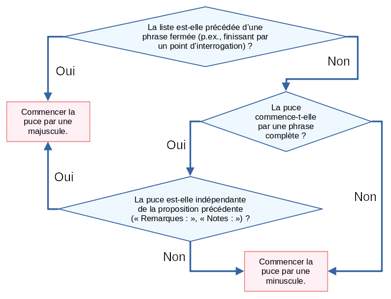
Essayons de construire un algorithme qui nous permet de trouver à coup sûr quelle casse et quelle ponctuation utiliser. Commençons par la casse de début d’élément.
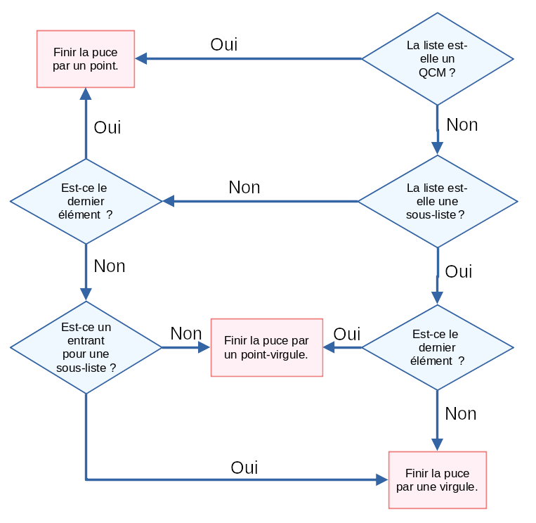
Nous pouvons ensuite nous tourner vers la ponctuation terminant les entrées. Notons que je ne considère ici qu’un seul niveau d’imbrication. L’algorithme pourrait être généralisé en remplaçant points-virgules et virgules par ponctuation ouverte de niveau n et n+1.
Et voilà ! Vous pouvez maintenant être confiant·e dans le formatage de votre liste !
Tout le monde connaît les faux-amis anglais-français comme actually et actuellement, le second signifiant « maintenant » tandis que le premier signifie « en réalité ». Mais certains faux-amis sont plus rares ou plus subtils. En voici quelques-uns auxquels un traducteur doit faire attention. Je mettrai cette liste à jour au fur et à mesure que j’en rencontrerai de nouveaux.
Agenda et agenda
En français un agenda est un petit livre contenants des pages correspondant à chaque jour, destiné à enregistrer les activités et rendez-vous à venir. La traduction anglaise est diary. En anglais, un agenda est soit une liste de chose à faire (ce que l’on écrirait dans un agenda français), c’est-à-dire un ordre du jour, soit un but caché.
Bigot et bigot
En français, un bigot ou une bigote sont des croyants pratiquants à l’extrême, des « grenouilles de bénitier ». En anglais, le terme n’est pas limité à la religion. A bigot est une personne extrêmement attachée à une idée, et ayant des préjugé ou même une attitude agressive envers toute personne ne partageant pas cette croyance.
Mettre les points sur les i et dotting the i’s
En français, mettre les points sur les i signifie être clair avec quelqu’un qui ne veut pas comprendre. Une expression très proche (que l’on utilisera toutefois dans un contexte légèrement différent) est remettre les pendules à l’heure. Une traduction en anglais serait to set the record straight. En revanche l’expression anglaise dotting the i’s signifie clarifier tous les détails, fignoler un travail. On l’utilise souvent dans l’expression plus longue dotting the i’s and crossing the t’s.
Adresser et to address
Tout comme le verbe anglais to address, le verbe français adresser possède un grand nombre d’acceptions dont certaines sont partagées. « To address a letter » signifie « adresser une lettre ». « To address someone » signifie « s’adresser à quelqu’un » Cependant, l’un comme l’autre présente des significations qui lui sont propres. Attention donc aux faux-amis. « to address a problem or a question » se traduit par « s’occuper d’un problème » ou « répondre à une question ». Pour répondre à des questions métaphysiques, on peut « s’adresser à la philosophie », qui en anglais se traduira pas « to turn to phylosophy ».
Déception et deception
En anglais, une deception est un mensonge, une tromperie, une action visant à induire quelqu’un en erreur. Cette signification a disparu en français, où une déception est le sentiment la tristesse ressentit lorsqu’un espoir n’est pas rempli. La traduction anglaise de déception est disappointment.
Accord et accord
Dans le cadre d’un traitement, un le français accord correspond à l’anglais assent (donner son accord). En anglais, un accord est une adhésion thérapeutique, une convergence de vue avec la personne prescrivant le traitement (les opinions sont en accord).
Cave et cave
En français, la cave est une pièce en sous-sol, par exemple pour conserver le vin, et se traduit par cellar en anglais. En anglais, a cave est un trou dans un relief rocheux, traduit par caverne ou grotte en français.
Mental et mental
En anatomie, l’adjectif anglais mental se réfère au menton (du latin mentum), comme dans « mental foramen ». En français, l’adjectif correct est mentonnier, mental faisant référence au latin mens, l’esprit.
Crâne et crane
En anglais, crane signifie grue, que ce soit l’oiseau ou la machine. Le français, crâne se traduit par l’anglais skull.
Lunatique et lunatic
En anglais, une personne lunatic est un·e fo·u·olle (loony), tandis qu’en français un lunatique est quelqu’un qui change d’opinion sur un coup de tête.
Dramatique et dramatic
En anglais, dramatic peut signifier « soudain et frappant » et avoir une connotation positive (par exemple, « a dramatic increase of cancer remissions »). L’utilisation du français dramatique ici impliquerait une tragédie avec des conséquences très négatives. La traduction française correcte est spectaculaire, « une augmentation spectaculaire des rémissions de cancer ».
Diaphorétique et diaphoretic
Assez technique et subtil, mais sémantiquement et médicalement important. L’adjectif français diaphorétique signifie uniquement « qui fait transpirer », tandis que l’adjectif anglais diaphoretic signifie également « transpirer excessivement », tant pour une personne que pour une peau.
Adhésion (thérapeutique) et (medical) adherence
En anglais, l’adherence d’un patient est le respect scrupuleux d’un traitement, y compris la posologie des médicaments, le calendrier d’administration et toute autre mesure prescrite. Elle est traduite par le français observance. Alors qu’en français, l’adhésion thérapeutique correspond à l’anglais concordance lorsque le patient est d’accord avec le choix fait et les décisions prises par le personnel de santé, et qu’il devient un participant actif de son traitement. Notez qu’en français, adhésion et adhérence sont utilisées dans des contextes différents.
Affecter et to affect
L’anglais to affect, qui signifie avoir un effet sur quelque chose, est (devrait être) traduit par influer sur. Le français affecter signifie adopter, prétendre si l’on parle de l’attitude d’une personne, et présenter si l’on parle des caractéristiques d’une chose.
Fastidieux et fastidious
En français, fastidieux présente une connotation négative, décrivant quelque chose de répétitif et d’ennuyeux. La traduction anglaise est tedious. Au contraire, en anglais, fastidious peut avoir une connotation positive, décrivant quelqu’un qui se soucie de la précision et des détails, correspondant au français pointilleux.
Légume et legume
En anglais, un legume est une plante (ou son fruit) appartenant à la famille des Leguminosae, comme les haricots, les pois, les cacahuètes ou les lentilles. La traduction française est légumineuse. En français, un légume est toute plante potagère cultivée pour l’alimentation, correspondant à l’anglais vegetable. En français, un végétal est toute plante, champignon ou algue.
Vocable et vocable
En anglais, un vocable est un énoncé non verbal, tel que « la la la », « Huh », etc. À l’opposé, en français, un vocable est un mot ou une expression dont la sémantique est très précise, parfois contextuelle.
Employé et employee
En anglais, un employee est une personne payée par une autre pour fournir un travail. En français, les employés forment une catégorie de travailleurs dont le travail n’est pas manuel, mais qui n’occupent pas une position de cadre. La traduction française correcte d’employee est salarié.
Idiome et idiom
En français, idiome signifie dialecte. En anglais, un idiom est une expression dont le sens est figuratif. La traduction française d’idiom est idiotisme. En anglais, l’idiotism est la condition rendant idiot.
Criquet et cricket
La traduction française de l’anglais cricket est grillon. Le criquet français est traduit en anglais par grasshopper. En fait, les Français ont volé le nom anglais pour nommer par erreur tous les insectes du sous-ordre Caelifera. Ceux-ci sont divisés en locustes s’ils peuvent former des populations migrantes et en sauteriaux s’ils ne le peuvent pas. Là, où cela devient amusant, c’est que locuste est le latin pour sauterelle. Par conséquent, les criquets français sont divisés en sauteriaux et en sauterelles !
Pétulant et petulant
Petulant en anglais et pétulant en français ont des significations légèrement différentes. L’ancienne dirigeante des libéraux démocrates,Jo Swinson, a été traitée de petulant par un député travailliste. Il voulait dire par là qu’elle avait mauvais caractère, était boudeuse. En français, pétulante signifie dynamique, plein d’énergie, ce qu’était aussi Jo Swinson… peut-être un peu trop.
Everyone knows English-French “false friends” such as actually and actuellement, the second meaning “currently” while the first means “in reality”. But some false friends are rarer or subtler. Below are a few of them that a translator should worry about. I will update the list as I come across new ones.
Agenda versus agenda
In English, an agenda is either a list of things to be discussed or done, an ordre du jour in French, or a hidden plan. While in French, an agenda is the physical support on which to write down the things to be discussed or done, i.e., a diary.
Bigot versus bigot
In English, a bigot is a person extremely attached to an idea, and prejudice or even antagonistic with anyone who is not sharing this belief. In France, the term is reserved for religion, unbigot or unebigote being religious believers whose practice is extreme.
Dotting the i’s versus mettre les points sur les i
In English, dotting the i’s means to finish something to perfection. It is often used as part ofdotting the i’s and crossing the t’s.The French translation would be fignoler [un travail]. However, the French expression mettre les points sur les i means to be very clear with someone who is reluctant to understand. An English translation would beto set the record straight.
To address versus adresser
Like the English verb to address, the French verb adresser has many meanings, some of which are shared. “To address a letter” means “adresser une lettre”. “To address someone” means “s’adresser à quelque’un”. However, both also present specific meanings. So beware of false friends. “To address a problem or a question” is translated into “s’occuper d’un problème” or “répondre à une question”. To answer metaphysical questions, one can, in French, “s’adresser à la philosophie”, which in English is translated as “to turn to phylosophy”.
Deception versus déception
In English, a “deception” is a lie, a sham, an action aimed at misleading someone. This meaning has disappeared in French, where a “déception” is the feeling of sadness felt when a hope is not fulfilled. The English translation of “déception” is “disappointment”.
Accord versus accord
In the context of treatment, an accord in French is an assent in English (to give one’s assent). An accord in English is an adherence, a congruence of views with the person prescribing the treatment (opinions are accorded).
Cave versus cave
In French, la cave is a room in the basement, for example for storing wine, and is translated as cellar in English. In English, a cave is a hole in a rocky outcrop, translated as caverne or grotte in French.
Mental versus mental
In anatomy, the English adjective mental refers to the chin (from Latin mentum), as in “mental foramen”. In French, the correct adjective is mentonnier, mental referring to the Latin mens, the mind.
Crane versus crâne
The English crane corresponds to the French grue, whether it is the bird or the machine. The French crâne is translated as skull.
Lunatic versus lunatique
In English, a lunatic person is crazy (loony), while in French a lunatique is someone who changes their opinion on a whim.
Dramatic versus dramatique
In English, dramatic can mean “sudden and striking” and be very positive (e.g., a dramatic increase of cancer remissions). Using the French dramatique here would imply a tragedy with very negative consequences. The proper French translation is spectaculaire, “une augmentation spectaculaire des rémissions de cancer”.
Diaphoretic versus diaphorétique
Quite technical and subtle, but semantically and medically significant. The French adjective diaphorétique only means “that causes perspiration”, while the English adjective diaphoretic also means “perspiring excessively”, both for a person or a skin.
(medical)Adherence versus adhésion(thérapeutique)
In English, a patient’s adherence to treatment is careful compliance with the treatment regimen, including drug dosing, schedule, and other prescribed measures. It is translated by the French observance. While the French adhésion thérapeutique corresponds to the English concordance between the patient and the health care professional when the patient is on-board with the choice made and the decisions taken, and became an active participant in their treatment. Note that in French, adhésion and adhérence are used in different contexts.
To affect versus affecter
The English to affect, meaning to have an effect on something, is (should be) translated by influersur. The French affecter means to adopt, to pretend if we are talking about a person’s attitude, and to present if we are talking about the features of a thing.
Fastidious versus fastidieux
In French, fastidieux has a negative overtone, describing something repetitive and boring. The English translation is tedious. On the contrary, in English, fastidious may have a positive overtone, describing someone who cares about accuracy and the details, corresponding to the French pointilleux.
legumeversuslégume
In English, a legume is a plant (or its fruit) belonging to the Leguminosae family, such as beans, peas, peanuts, or lentils. The French translation is légumineuse. In French, a légume is any garden plant cultivated for nutrition, corresponding to English vegetable. In French, a végétal is any plant, mushroom, or alga.
Vocableversusvocable
In English, a vocable is a non-word utterance, such as “la la la”, “Huh”, etc. Now let’s U-turn, in French, a vocable is a word or an expression with very precise, sometimes contextual, semantics.
Employeeversusemployé
In English, an employee is someone paid by someone else to work for them. In French, employés is a category of workers, whose work is not manual and who are not in a managing position. The correct French translation of employee is salarié.
Idiomversusidiome
In French, idiome means dialect. In English, idiom is an expression with a non-literal meaning. The French version of idiom is idiotisme. In English, idiotism is the condition to be an idiot.
Cricketversuscriquet
The French translation of English cricket is grillon. The French criquet is translated into English by grasshopper. In fact, the French stole the English name to mistakenly name all insects of the suborder Caelifera. These are divided into locustes if they can form migrant populations and in sauteriaux if they cannot. Now, the interesting bit is that locuste is the latin name for sauterelle. Therefore, the French criquets are divided in sauteriaux and sauterelles!
Petulantversuspétulant
Petulant in English and pétulant in French have slightly different meanings. The once liberal democrat leader Jo Swinson was called petulant by a labour frontbencher. He meant it as bad-tempered, sulky. In French, pétulant means dynamic, full of energy, which is also what Jo Swinson was… perhaps a bit too much.
Comme nous l’a montré le déluge de communication autour des vaccins contre la covid-19, la terminologie de pharmacovigilance (le suivi de la sécurité des médicaments, à savoir leur innocuité et leur tolérabilité) peut entraîner de la confusion, voire nourrir les acteurs de la désinformation. l’Organisation mondiale de la santé (OMS) fournit des définitions claires de termes précis qui sont malheureusement souvent détournés de leur sens premier.
Les événements indésirables (adverse event en anglais) recouvrent tout ce dont souffrent les personnes dans les périodes suivant l’administration d’un traitement (qu’il soit prophylactique ou thérapeutique). Les périodes concernées peuvent varier très largement. Un des principaux outils de pharmacovigilance est le recueil des signalements de tels événements indésirable. C’est par exemple le rôle du VAERS (Vaccine Adverse Event Reporting System) des Centers for Disease Control and Prevention (CDC) et de la Food and Drug Administration (FDA) aux États-unis, de l’ANSM (Agence nationale de sécurité du médicament et des produits de santé) en France, ou encore de la MHRA (Medicines & Healthcare products Regulatory Agency) au Royaume-Uni. La survenue ou l’incidence de ces événements ne sont pas nécessairement liées au traitement. Par exemple, dans les cas des vaccins contre la covid-19, la MHRA répertoriait les chutes, les électrocutions, les morsures d’insectes et les accidents de voitures. Bien que l’incidence de ces événements puisse être affectée par certains médicaments, il est peu probable que ce soit le cas pour des vaccins.
Si l’événement peut engager le pronostic vital, on parle d’événement indésirable grave (serious adverse event en anglais). Rappelons la différence entre sévère et grave (severe et serious en anglais). La sévérité est liée à l’intensité d’un phénomène. La gravité est liée aux conséquences de ce phénomène. Un symptôme ou un signe clinique peut être sévère sans être avoir de conséquences majeurs sur la santé et vice-versa. À noter que la gravité dépend du contexte personnel et environnemental. Selon les antécédents du patient et ses circonstances, un événement peut être bénin ou grave.
Quand l’événement indésirable est prouvé être directement en rapport avec le traitement, qu’il soit entraîné par le traitement lui-même ou par les circonstances de son administration, on parle d’événement indésirable associé aux soins (treatment-emergent adverse event en anglais)
Un effet indésirable (adverse effect ou adverse reaction en anglais) est un événement indésirable directement causé par le traitement. Il est à noter que tous les événements indésirables d’un certain type ne sont pas dus au traitement et donc des effets indésirable. Par exemple, les événements thromboemboliques et les myocardites sont des événements relativement fréquents et qui sont parmi les complications principales de la covid-19. Bien que les vaccins à adénovirus et à ARNm, respectivement, aient montré un accroissement de leur incidence dans certaines populations, des analyses statistiques poussées ont été nécessaires
Un effet secondaire (side effect en anglais) est un effet directement dû au traitement, mais qui n’est pas nécessairement indésirable. Par exemple, l’inhibition de l’agrégation plaquettaire par l’aspirine est utilisée pour prévenir la formation de caillots sanguins.